

8
1 Introduction
P
(2)
p (t) =
t
−∞
dt
t
−∞
dt
x−z
q,r
χ
(2)
pqr (t, t
, t
)E q (t
)E r (t
)
(1.2)
=
k
l
t
−∞
dt
t
−∞
dt
x−z
q,r
χ
(2)
pqr (t, t
, t
)E q (ω k )E r (ω l )
exp(−iω k t
) exp(−iω l t
).
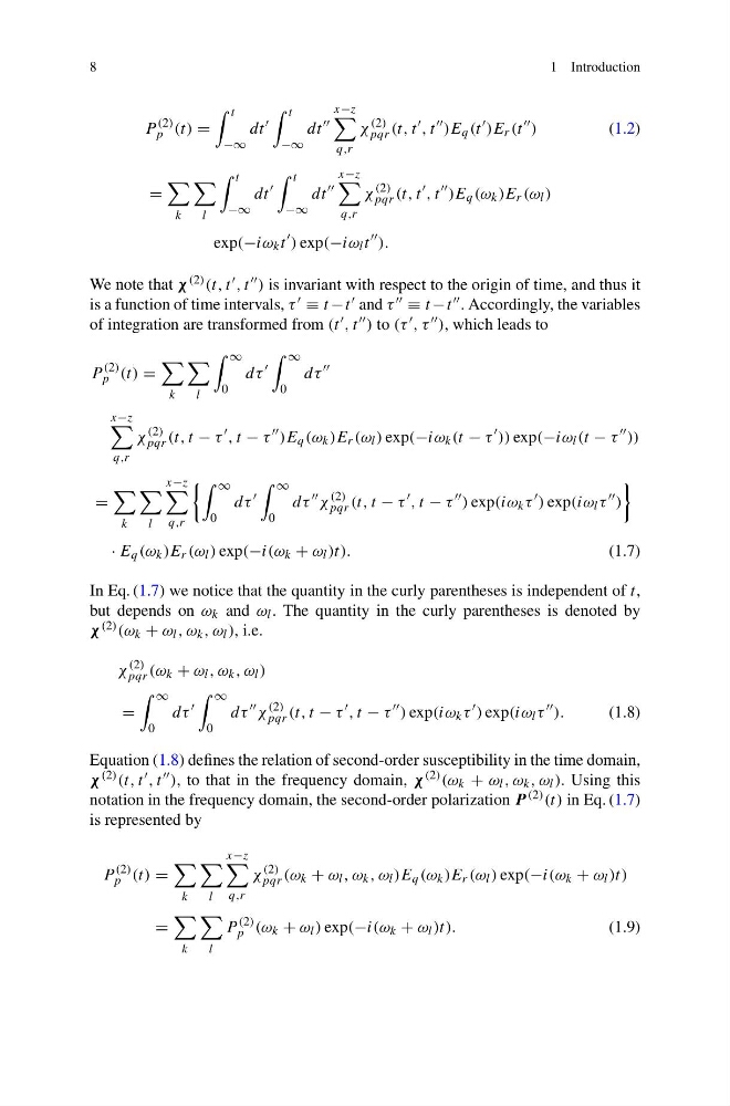
We note that χ (2) (t, t , t ) is invariant with respect to the origin of time, and thus it
is a function of time intervals, τ ≡ t −t and τ ≡ t −t . Accordingly, the variables
of integration are transformed from (t , t ) to (τ , τ ), which leads to
P
(2)
p (t) =
k
l
∞
0
dτ
∞
0
dτ
x−z
q,r
χ
(2)
pqr (t, t − τ
, t − τ
)E q (ω k )E r (ω l ) exp(−iω k (t − τ
)) exp(−iω l (t − τ
))
=
k
l
x−z
q,r
∞
0
dτ
∞
0
dτ
χ
(2)
pqr (t, t − τ
, t − τ
) exp(iω k τ
) exp(iω l τ
)
· E q (ω k )E r (ω l ) exp(−i(ω k + ω l )t).
(1.7)
In Eq. (1.7) we notice that the quantity in the curly parentheses is independent of t,
but depends on ω k and ω l . The quantity in the curly parentheses is denoted by
χ (2) (ω k + ω l , ω k , ω l ), i.e.
χ
(2)
pqr (ω k + ω l , ω k , ω l )
=
∞
0
dτ
∞
0
dτ
χ
(2)
pqr (t, t − τ
, t − τ
) exp(iω k τ
) exp(iω l τ
).
(1.8)
Equation (1.8) defines the relation of second-order susceptibility in the time domain,
χ (2) (t, t , t ), to that in the frequency domain, χ (2) (ω k + ω l , ω k , ω l ). Using this
notation in the frequency domain, the second-order polarization P (2) (t) in Eq. (1.7)
is represented by
P
(2)
p (t) =
k
l
x−z
q,r
χ
(2)
pqr (ω k + ω l , ω k , ω l )E q (ω k )E r (ω l ) exp(−i(ω k + ω l )t)
=
k
l
P
(2)
p (ω k + ω l ) exp(−i(ω k + ω l )t).
(1.9)
1 Introduction
P
(2)
p (t) =
t
−∞
dt
t
−∞
dt
x−z
q,r
χ
(2)
pqr (t, t
, t
)E q (t
)E r (t
)
(1.2)
=
k
l
t
−∞
dt
t
−∞
dt
x−z
q,r
χ
(2)
pqr (t, t
, t
)E q (ω k )E r (ω l )
exp(−iω k t
) exp(−iω l t
).
We note that χ (2) (t, t , t ) is invariant with respect to the origin of time, and thus it
is a function of time intervals, τ ≡ t −t and τ ≡ t −t . Accordingly, the variables
of integration are transformed from (t , t ) to (τ , τ ), which leads to
P
(2)
p (t) =
k
l
∞
0
dτ
∞
0
dτ
x−z
q,r
χ
(2)
pqr (t, t − τ
, t − τ
)E q (ω k )E r (ω l ) exp(−iω k (t − τ
)) exp(−iω l (t − τ
))
=
k
l
x−z
q,r
∞
0
dτ
∞
0
dτ
χ
(2)
pqr (t, t − τ
, t − τ
) exp(iω k τ
) exp(iω l τ
)
· E q (ω k )E r (ω l ) exp(−i(ω k + ω l )t).
(1.7)
In Eq. (1.7) we notice that the quantity in the curly parentheses is independent of t,
but depends on ω k and ω l . The quantity in the curly parentheses is denoted by
χ (2) (ω k + ω l , ω k , ω l ), i.e.
χ
(2)
pqr (ω k + ω l , ω k , ω l )
=
∞
0
dτ
∞
0
dτ
χ
(2)
pqr (t, t − τ
, t − τ
) exp(iω k τ
) exp(iω l τ
).
(1.8)
Equation (1.8) defines the relation of second-order susceptibility in the time domain,
χ (2) (t, t , t ), to that in the frequency domain, χ (2) (ω k + ω l , ω k , ω l ). Using this
notation in the frequency domain, the second-order polarization P (2) (t) in Eq. (1.7)
is represented by
P
(2)
p (t) =
k
l
x−z
q,r
χ
(2)
pqr (ω k + ω l , ω k , ω l )E q (ω k )E r (ω l ) exp(−i(ω k + ω l )t)
=
k
l
P
(2)
p (ω k + ω l ) exp(−i(ω k + ω l )t).
(1.9)