

134
6 Charge Response Kernel for Electronic Polarization
6.4 χ (2) Formula with CRK Model
Then we present the χ (2) formula based on the CRK model. We have derived χ (2) in
Sect. 5.2 with the time correlation function of A eff and M in Eq. (5.27). The purpose
here is to express A eff and M using the CRK model. The following derivation with
the CRK model provides an alternative but physically equivalent treatment of the
local field effect in Sect. 5.
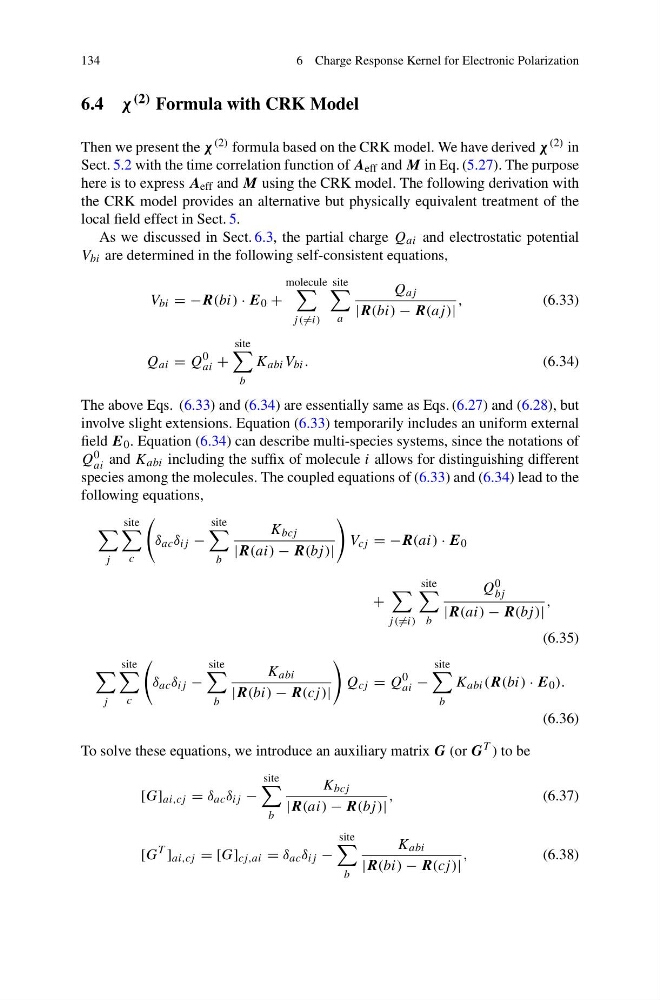
As we discussed in Sect. 6.3, the partial charge Q ai and electrostatic potential
V bi are determined in the following self-consistent equations,
V bi = −R(bi) · E 0 +
molecule
j ( =i)
site
a
Q aj
|R(bi) − R(aj )|
,
(6.33)
Q ai = Q
0
ai +
site
b
K abi V bi .
(6.34)
The above Eqs. (6.33) and (6.34) are essentially same as Eqs. (6.27) and (6.28), but
involve slight extensions. Equation (6.33) temporarily includes an uniform external
field E 0 . Equation (6.34) can describe multi-species systems, since the notations of
Q 0
ai and K abi including the suffix of molecule i allows for distinguishing different
species among the molecules. The coupled equations of (6.33) and (6.34) lead to the
following equations,
j
site
c
δ ac δ ij −
site
b
K bcj
|R(ai) − R(bj )|
V cj = −R(ai) · E 0
+
j ( =i)
site
b
Q 0
bj
|R(ai) − R(bj )|
,
(6.35)
j
site
c
δ ac δ ij −
site
b
K abi
|R(bi) − R(cj )|
Q cj = Q
0
ai −
site
b
K abi (R(bi) · E 0 ).
(6.36)
To solve these equations, we introduce an auxiliary matrix G (or G
T ) to be
[G] ai,cj = δ ac δ ij −
site
b
K bcj
|R(ai) − R(bj )|
,
(6.37)
[G
T
] ai,cj = [G] cj,ai = δ ac δ ij −
site
b
K abi
|R(bi) − R(cj )|
,
(6.38)
6 Charge Response Kernel for Electronic Polarization
6.4 χ (2) Formula with CRK Model
Then we present the χ (2) formula based on the CRK model. We have derived χ (2) in
Sect. 5.2 with the time correlation function of A eff and M in Eq. (5.27). The purpose
here is to express A eff and M using the CRK model. The following derivation with
the CRK model provides an alternative but physically equivalent treatment of the
local field effect in Sect. 5.
As we discussed in Sect. 6.3, the partial charge Q ai and electrostatic potential
V bi are determined in the following self-consistent equations,
V bi = −R(bi) · E 0 +
molecule
j ( =i)
site
a
Q aj
|R(bi) − R(aj )|
,
(6.33)
Q ai = Q
0
ai +
site
b
K abi V bi .
(6.34)
The above Eqs. (6.33) and (6.34) are essentially same as Eqs. (6.27) and (6.28), but
involve slight extensions. Equation (6.33) temporarily includes an uniform external
field E 0 . Equation (6.34) can describe multi-species systems, since the notations of
Q 0
ai and K abi including the suffix of molecule i allows for distinguishing different
species among the molecules. The coupled equations of (6.33) and (6.34) lead to the
following equations,
j
site
c
δ ac δ ij −
site
b
K bcj
|R(ai) − R(bj )|
V cj = −R(ai) · E 0
+
j ( =i)
site
b
Q 0
bj
|R(ai) − R(bj )|
,
(6.35)
j
site
c
δ ac δ ij −
site
b
K abi
|R(bi) − R(cj )|
Q cj = Q
0
ai −
site
b
K abi (R(bi) · E 0 ).
(6.36)
To solve these equations, we introduce an auxiliary matrix G (or G
T ) to be
[G] ai,cj = δ ac δ ij −
site
b
K bcj
|R(ai) − R(bj )|
,
(6.37)
[G
T
] ai,cj = [G] cj,ai = δ ac δ ij −
site
b
K abi
|R(bi) − R(cj )|
,
(6.38)