

116
5 Molecular Theory of Local Field
E
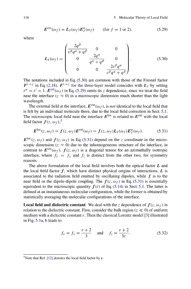
ext (ω f ) = L I (ω f )E
α
I (ω f )
(for f = 1 or 2),
(5.29)
where
L I (ω f ) =
⎛
⎜
⎜
⎜
⎜
⎜
⎜
⎝
2q β
ε β q α + q β
0
0
0
2q α
q α + q β
0
0
0
2ε β q α
ε β q α + q β
⎞
⎟
⎟
⎟
⎟
⎟
⎟
⎠
.
(5.30)
The notations included in Eq. (5.30) are common with those of the Fresnel factor
F i→j in Eq. (2.18). F i→j for the three-layer model coincides with L I by setting
ε α = ε = 1. E ext (ω f ) in Eq. (5.29) omits its z dependence, since we treat the field
near the interface (z ≈ 0) in a microscopic dimension much shorter than the light
wavelength.
The external field at the interface, E ext (ω f ), is not identical to the local field that
is felt by an individual molecule there, due to the local field correction in Sect. 5.1.
The microscopic local field near the interface E loc is related to E ext with the local
field factor f (z, ω f ), 5
E
loc (z, ω f ) = f (z, ω f )E
ext (ω f ) = f (z, ω f )L I (ω f )E
α
I (ω f ).
(5.31)
E loc (z, ω f ) and f (z, ω f ) in Eq. (5.31) depend on the z coordinate in the microscopic dimension (z ≈ 0) due to the inhomogeneous structure of the interface, in
contrast to E ext (ω f ). f (z, ω f ) is a diagonal tensor for an azimuthally isotropic
interface, where f x = f y and f z is distinct from the other two, for symmetry
reasons.
The above formulation of the local field involves both the optical factor L and
the local field factor f , which have distinct physical origins of interactions. L is
associated to the radiation field emitted by oscillating dipoles, while f is to the
near field or the dipole-dipole coupling. The f (z, ω f ) in Eq. (5.31) is essentially
equivalent to the microscopic quantity f (i) of Eq. (5.14) in Sect. 5.1. The latter is
defined at an instantaneous molecular configuration, while the former is obtained by
statistically averaging the molecular configurations of the interface.
Local field and dielectric constant We deal with the z dependence of f (z, ω f ) in
relation to the dielectric constant. First, consider the bulk region (z 0) of uniform
medium with a dielectric constant ε. Then the classical Lorentz model [3] illustrated
in Fig. 5.1a, b leads to
f x = f y =
ε + 2
3
and f z =
ε + 2
3ε
.
(5.32)
5 Note that Ref. [12] denotes the local field factor by s.
5 Molecular Theory of Local Field
E
ext (ω f ) = L I (ω f )E
α
I (ω f )
(for f = 1 or 2),
(5.29)
where
L I (ω f ) =
⎛
⎜
⎜
⎜
⎜
⎜
⎜
⎝
2q β
ε β q α + q β
0
0
0
2q α
q α + q β
0
0
0
2ε β q α
ε β q α + q β
⎞
⎟
⎟
⎟
⎟
⎟
⎟
⎠
.
(5.30)
The notations included in Eq. (5.30) are common with those of the Fresnel factor
F i→j in Eq. (2.18). F i→j for the three-layer model coincides with L I by setting
ε α = ε = 1. E ext (ω f ) in Eq. (5.29) omits its z dependence, since we treat the field
near the interface (z ≈ 0) in a microscopic dimension much shorter than the light
wavelength.
The external field at the interface, E ext (ω f ), is not identical to the local field that
is felt by an individual molecule there, due to the local field correction in Sect. 5.1.
The microscopic local field near the interface E loc is related to E ext with the local
field factor f (z, ω f ), 5
E
loc (z, ω f ) = f (z, ω f )E
ext (ω f ) = f (z, ω f )L I (ω f )E
α
I (ω f ).
(5.31)
E loc (z, ω f ) and f (z, ω f ) in Eq. (5.31) depend on the z coordinate in the microscopic dimension (z ≈ 0) due to the inhomogeneous structure of the interface, in
contrast to E ext (ω f ). f (z, ω f ) is a diagonal tensor for an azimuthally isotropic
interface, where f x = f y and f z is distinct from the other two, for symmetry
reasons.
The above formulation of the local field involves both the optical factor L and
the local field factor f , which have distinct physical origins of interactions. L is
associated to the radiation field emitted by oscillating dipoles, while f is to the
near field or the dipole-dipole coupling. The f (z, ω f ) in Eq. (5.31) is essentially
equivalent to the microscopic quantity f (i) of Eq. (5.14) in Sect. 5.1. The latter is
defined at an instantaneous molecular configuration, while the former is obtained by
statistically averaging the molecular configurations of the interface.
Local field and dielectric constant We deal with the z dependence of f (z, ω f ) in
relation to the dielectric constant. First, consider the bulk region (z 0) of uniform
medium with a dielectric constant ε. Then the classical Lorentz model [3] illustrated
in Fig. 5.1a, b leads to
f x = f y =
ε + 2
3
and f z =
ε + 2
3ε
.
(5.32)
5 Note that Ref. [12] denotes the local field factor by s.