

5.1 Local Field Correction Factor
109
The left side consists of the “external” field E 0 and the electric field from permanent
dipoles of neighboring molecules −T μ 0 . E 0 −T μ 0 is a hypothetical electric field in
Eq. (5.7) with the polarizability switched off, α = 0. In the realistic case, however,
the dipole moments of molecules are affected each other, and as a consequence,
the electric field changes from E 0 − T μ 0 to E. g is therefore considered to be a
microscopic definition of the local field correction factor, and deviates from unity
when the constituent molecules are polarizable.
In the same vein, Eq. (5.10) illustrates the role of g T , which changes the dipole
moments of molecules from μ 0 to μ,
μ
0
+ αE
0
= μ
0 g T
− → μ.
The left side μ 0 stands for the dipole moment consisting of the permanent dipole
μ 0 and the induced one by the external field αE 0 . Accordingly, μ 0 does not include
the dipole-dipole interaction among molecular polarizations, and g T takes account
of the dipole-dipole coupling effect on the polarizations. To summarize, both factors
g and g T account for the effect of the self-consistent coupling among polarizations.
g affects on the electric field while g T on the dipole moment. Note the distinction
between g and g T in the transpose relation.
Dipole M Using the solutions of E and μ in Eqs. (5.9) and (5.10), we can derive
the dipole moment and polarizability of the whole system. The dipole moment of
the whole system M is given by the sum of total (permanent + induced) dipole
moments of constituent molecules,
M =
N
i=1
μ(i).
(5.12)
μ(i) is a part of the 3N -dimensional vector μ in Eq. (5.5). Equation (5.12) is
expanded in the component representation using Eq. (5.10) by
M p =
N
i=1
μ p (i) =
N
i,j
x∼z
q
g
T
pq (ij )
μ
0
q (j ) +
x∼z
r
α qr (j )E
0
r (j )
=
N
i,j
x∼z
q
g
T
pq (ij )μ
0
q (j ) =
i,j
x∼z
q
μ
0
q (j )g qp (j i) =
N
j =1
x∼z
q
μ
0
q (j )f qp (j ).
(5.13)
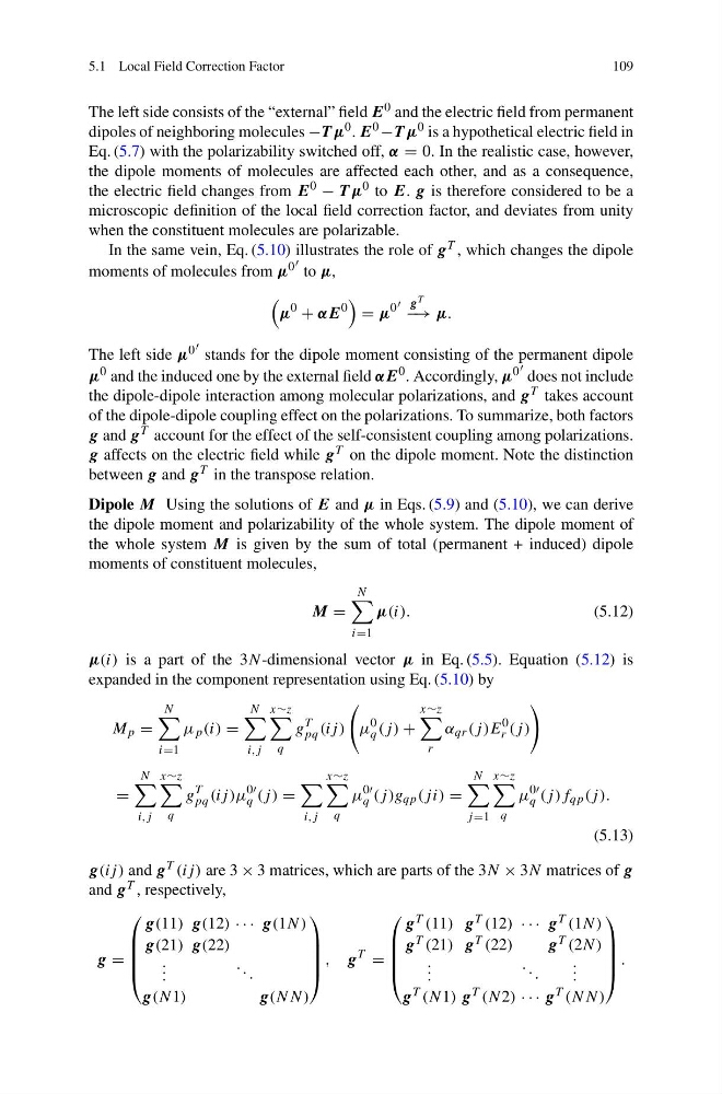
g(ij ) and g T (ij ) are 3 × 3 matrices, which are parts of the 3N × 3N matrices of g
and g T , respectively,
g =
⎛
⎜
⎜
⎜
⎝
g(11) g(12) · · · g(1N)
g(21) g(22)
. . .
. . .
g(N1)
g(NN)
⎞
⎟
⎟
⎟
⎠
, g
T
=
⎛
⎜
⎜
⎜
⎝
g T (11) g T (12) · · · g T (1N)
g T (21) g T (22)
g T (2N)
. . .
. . .
. . .
g T (N1) g T (N2) · · · g T (NN)
⎞
⎟
⎟
⎟
⎠
.
109
The left side consists of the “external” field E 0 and the electric field from permanent
dipoles of neighboring molecules −T μ 0 . E 0 −T μ 0 is a hypothetical electric field in
Eq. (5.7) with the polarizability switched off, α = 0. In the realistic case, however,
the dipole moments of molecules are affected each other, and as a consequence,
the electric field changes from E 0 − T μ 0 to E. g is therefore considered to be a
microscopic definition of the local field correction factor, and deviates from unity
when the constituent molecules are polarizable.
In the same vein, Eq. (5.10) illustrates the role of g T , which changes the dipole
moments of molecules from μ 0 to μ,
μ
0
+ αE
0
= μ
0 g T
− → μ.
The left side μ 0 stands for the dipole moment consisting of the permanent dipole
μ 0 and the induced one by the external field αE 0 . Accordingly, μ 0 does not include
the dipole-dipole interaction among molecular polarizations, and g T takes account
of the dipole-dipole coupling effect on the polarizations. To summarize, both factors
g and g T account for the effect of the self-consistent coupling among polarizations.
g affects on the electric field while g T on the dipole moment. Note the distinction
between g and g T in the transpose relation.
Dipole M Using the solutions of E and μ in Eqs. (5.9) and (5.10), we can derive
the dipole moment and polarizability of the whole system. The dipole moment of
the whole system M is given by the sum of total (permanent + induced) dipole
moments of constituent molecules,
M =
N
i=1
μ(i).
(5.12)
μ(i) is a part of the 3N -dimensional vector μ in Eq. (5.5). Equation (5.12) is
expanded in the component representation using Eq. (5.10) by
M p =
N
i=1
μ p (i) =
N
i,j
x∼z
q
g
T
pq (ij )
μ
0
q (j ) +
x∼z
r
α qr (j )E
0
r (j )
=
N
i,j
x∼z
q
g
T
pq (ij )μ
0
q (j ) =
i,j
x∼z
q
μ
0
q (j )g qp (j i) =
N
j =1
x∼z
q
μ
0
q (j )f qp (j ).
(5.13)
g(ij ) and g T (ij ) are 3 × 3 matrices, which are parts of the 3N × 3N matrices of g
and g T , respectively,
g =
⎛
⎜
⎜
⎜
⎝
g(11) g(12) · · · g(1N)
g(21) g(22)
. . .
. . .
g(N1)
g(NN)
⎞
⎟
⎟
⎟
⎠
, g
T
=
⎛
⎜
⎜
⎜
⎝
g T (11) g T (12) · · · g T (1N)
g T (21) g T (22)
g T (2N)
. . .
. . .
. . .
g T (N1) g T (N2) · · · g T (NN)
⎞
⎟
⎟
⎟
⎠
.