

5.1 Local Field Correction Factor
107
where the suffixes p, q denote the space-fixed coordinates, x, y, or z. The first term
of the right-hand side of Eq. (5.1) means the permanent dipole moment of the i-th
molecule, and the second term the induced dipole. E(i) in Eq. (5.2) consists of two
terms. The field generated by the dipoles of neighboring molecules is represented
in the second term of the right-hand side of Eq. (5.2), while the first term E 0 (i)
accounts for the other sources of field than the dipole. T (ij) is called the dipoledipole coupling tensor, which describes the electric field at r(i) generated by a
dipole moment at r(j ). The explicit form of T pq (ij ) is 1
T pq (ij ) =
δ pq
r(ij )
3
−
3r p (ij )r q (ij )
r(ij )
5
,
(5.3)
where r(ij ) = |r(ij )| = |r(i) − r(j )|. Equations (5.1) and (5.2) define the
coupled relation between the dipole moment μ(i) and the electric field E(i), 2 and
accordingly both quantities should be solved simultaneously in a self-consistent
manner. In polarizable MD simulation, instantaneous polarizations of constituent
molecules are determined at each time step t self-consistently in this way. We
also note that E 0 in Eq. (5.2) includes the externally imposed field as well as the
intermolecular interactions other than the dipole-dipole coupling.
Solutions of μ and E Since Eqs. (5.1) and (5.2) are linear, the coupled equations
can be solved analytically. Equations (5.1) and (5.2) are written in the matrix form,
μ = μ
0
+ αE,
E = E
0
− T μ.
(5.4)
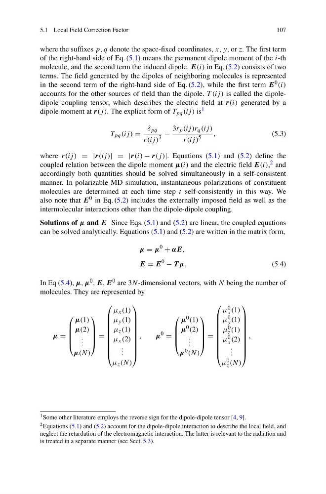
In Eq (5.4), μ, μ 0 , E, E 0 are 3N -dimensional vectors, with N being the number of
molecules. They are represented by
μ =
⎛
⎜
⎜
⎜
⎝
μ(1)
μ(2)
. . .
μ(N)
⎞
⎟
⎟
⎟
⎠
=
⎛
⎜
⎜
⎜
⎜
⎜
⎜
⎜
⎜
⎝
μ x (1)
μ y (1)
μ z (1)
μ x (2)
. . .
μ z (N)
⎞
⎟
⎟
⎟
⎟
⎟
⎟
⎟
⎟
⎠
,
μ
0
=
⎛
⎜
⎜
⎜
⎝
μ 0 (1)
μ 0 (2)
. . .
μ 0 (N)
⎞
⎟
⎟
⎟
⎠
=
⎛
⎜
⎜
⎜
⎜
⎜
⎜
⎜
⎜
⎝
μ 0
x (1)
μ 0
y (1)
μ 0
z (1)
μ 0
x (2)
. . .
μ 0
z (N)
⎞
⎟
⎟
⎟
⎟
⎟
⎟
⎟
⎟
⎠
,
1 Some other literature employs the reverse sign for the dipole-dipole tensor [4, 9].
2 Equations (5.1) and (5.2) account for the dipole-dipole interaction to describe the local field, and
neglect the retardation of the electromagnetic interaction. The latter is relevant to the radiation and
is treated in a separate manner (see Sect. 5.3).
107
where the suffixes p, q denote the space-fixed coordinates, x, y, or z. The first term
of the right-hand side of Eq. (5.1) means the permanent dipole moment of the i-th
molecule, and the second term the induced dipole. E(i) in Eq. (5.2) consists of two
terms. The field generated by the dipoles of neighboring molecules is represented
in the second term of the right-hand side of Eq. (5.2), while the first term E 0 (i)
accounts for the other sources of field than the dipole. T (ij) is called the dipoledipole coupling tensor, which describes the electric field at r(i) generated by a
dipole moment at r(j ). The explicit form of T pq (ij ) is 1
T pq (ij ) =
δ pq
r(ij )
3
−
3r p (ij )r q (ij )
r(ij )
5
,
(5.3)
where r(ij ) = |r(ij )| = |r(i) − r(j )|. Equations (5.1) and (5.2) define the
coupled relation between the dipole moment μ(i) and the electric field E(i), 2 and
accordingly both quantities should be solved simultaneously in a self-consistent
manner. In polarizable MD simulation, instantaneous polarizations of constituent
molecules are determined at each time step t self-consistently in this way. We
also note that E 0 in Eq. (5.2) includes the externally imposed field as well as the
intermolecular interactions other than the dipole-dipole coupling.
Solutions of μ and E Since Eqs. (5.1) and (5.2) are linear, the coupled equations
can be solved analytically. Equations (5.1) and (5.2) are written in the matrix form,
μ = μ
0
+ αE,
E = E
0
− T μ.
(5.4)
In Eq (5.4), μ, μ 0 , E, E 0 are 3N -dimensional vectors, with N being the number of
molecules. They are represented by
μ =
⎛
⎜
⎜
⎜
⎝
μ(1)
μ(2)
. . .
μ(N)
⎞
⎟
⎟
⎟
⎠
=
⎛
⎜
⎜
⎜
⎜
⎜
⎜
⎜
⎜
⎝
μ x (1)
μ y (1)
μ z (1)
μ x (2)
. . .
μ z (N)
⎞
⎟
⎟
⎟
⎟
⎟
⎟
⎟
⎟
⎠
,
μ
0
=
⎛
⎜
⎜
⎜
⎝
μ 0 (1)
μ 0 (2)
. . .
μ 0 (N)
⎞
⎟
⎟
⎟
⎠
=
⎛
⎜
⎜
⎜
⎜
⎜
⎜
⎜
⎜
⎝
μ 0
x (1)
μ 0
y (1)
μ 0
z (1)
μ 0
x (2)
. . .
μ 0
z (N)
⎞
⎟
⎟
⎟
⎟
⎟
⎟
⎟
⎟
⎠
,
1 Some other literature employs the reverse sign for the dipole-dipole tensor [4, 9].
2 Equations (5.1) and (5.2) account for the dipole-dipole interaction to describe the local field, and
neglect the retardation of the electromagnetic interaction. The latter is relevant to the radiation and
is treated in a separate manner (see Sect. 5.3).