

J. C. Dobrowolsk et al.
98
where
α
α
α
β
α
α
αα
ββ
αβ
α
i
i
i
i
i
Q
Q
Q
2
0
0
2
0
1
9
1
2
3
=
∂
∂
∂
∂
=
∂
∂
∂ β β
αα
ββ
α
α
β
∂
−
∂
∂
∂
∂
=
∂
Q
Q
Q
i
i
i
G i
0
0
0
2
1
2
3
α α
α
αβ
αβ
αα
ββ
∂
∂
∂
−
∂
∂
∂
∂
Q
G
Q
Q
G
Q
i
i
i
i
0
0
0
'
'
0 0
2
0
0
2
=
∂
∂
∂
∂
β
ω α
ε
αβ
αγδ
γδβ
A
i
i
i
i
Q
A
Q
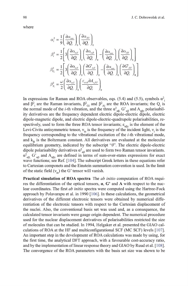
In expressions for Raman and ROA observables, eqs. (5.4) and (5.5), symbols α
2
i
and β
2
i
are the Raman invariants, β
2
gi
and β
2
Ai
are the RoA invariants; the Q i is
the normal mode of the i-th vibration, and the three α
2
αβ,
g’ αβ and A αβγ polarisability derivatives are the frequency dependent electric dipole-electric dipole, electric
dipole-magnetic dipole, and electric dipole-electric-quadrupole polarisabilities, respectively, used to form the three ROA tensor invariants; ε αβγ is the element of the
Levi-Civita antisymmetric tensor, ν in is the frequency of the incident light, ν i is the
frequency corresponding to the vibrational excitation of the i-th vibrational mode,
and k B is the Boltzmann constant. All derivatives are evaluated at the molecular
equilibrium geometry, indicated by the subscript “0”. the electric dipole-electric
dipole polarisability derivatives α
2
αβ
are used to form two Raman tensor invariants.
α
2
αβ,
g’ αβ and A αβγ are defined in terms of sum-over-states expressions for exact
wave functions; see Ref. [104]. the subscript greek letters in these equations refer
to Cartesian componets and the Einstein summation convention is used. In the limit
of the static field (ν in ) the g’ tensor will vanish.
Practical simulation of ROA spectra the ab initio computation of RoA requires the differentiation of the optical tensors, α, G’ and A with respect to the nuclear coordinates. the first ab initio spectra were computed using the hartree-Fock
approach by Polavarapu et al. in 1990 [106]. In these calculations, the geometrical
derivatives of the different electronic tensors were obtained by numerical differentiation of the electronic tensors with respect to the Cartesian displacement of
the nuclei. Also, the conventional basis set was used and, as a consequence, the
calculated tensor invariants were gauge origin dependent. the numerical procedure
used for the nuclear displacement derivatives of polarisabilities restricted the size
of molecules that can be studied. In 1994, helgaker et al. presented the gIAo calculations of RoA at the hF and multiconfigurational SCF (mC SCF) levels [107].
An important step in the development of RoA calculations was made by using, for
the first time, the analytical dFt approach, with a favourable cost-accuracy ratio,
and by the implementation of linear response theory and gIAo by Ruud et al. [108].
the convergence of the RoA parameters with the basis set size was shown to be
98
where
α
α
α
β
α
α
αα
ββ
αβ
α
i
i
i
i
i
Q
Q
Q
2
0
0
2
0
1
9
1
2
3
=
∂
∂
∂
∂
=
∂
∂
∂ β β
αα
ββ
α
α
β
∂
−
∂
∂
∂
∂
=
∂
Q
Q
Q
i
i
i
G i
0
0
0
2
1
2
3
α α
α
αβ
αβ
αα
ββ
∂
∂
∂
−
∂
∂
∂
∂
Q
G
Q
Q
G
Q
i
i
i
i
0
0
0
'
'
0 0
2
0
0
2
=
∂
∂
∂
∂
β
ω α
ε
αβ
αγδ
γδβ
A
i
i
i
i
Q
A
Q
In expressions for Raman and ROA observables, eqs. (5.4) and (5.5), symbols α
2
i
and β
2
i
are the Raman invariants, β
2
gi
and β
2
Ai
are the RoA invariants; the Q i is
the normal mode of the i-th vibration, and the three α
2
αβ,
g’ αβ and A αβγ polarisability derivatives are the frequency dependent electric dipole-electric dipole, electric
dipole-magnetic dipole, and electric dipole-electric-quadrupole polarisabilities, respectively, used to form the three ROA tensor invariants; ε αβγ is the element of the
Levi-Civita antisymmetric tensor, ν in is the frequency of the incident light, ν i is the
frequency corresponding to the vibrational excitation of the i-th vibrational mode,
and k B is the Boltzmann constant. All derivatives are evaluated at the molecular
equilibrium geometry, indicated by the subscript “0”. the electric dipole-electric
dipole polarisability derivatives α
2
αβ
are used to form two Raman tensor invariants.
α
2
αβ,
g’ αβ and A αβγ are defined in terms of sum-over-states expressions for exact
wave functions; see Ref. [104]. the subscript greek letters in these equations refer
to Cartesian componets and the Einstein summation convention is used. In the limit
of the static field (ν in ) the g’ tensor will vanish.
Practical simulation of ROA spectra the ab initio computation of RoA requires the differentiation of the optical tensors, α, G’ and A with respect to the nuclear coordinates. the first ab initio spectra were computed using the hartree-Fock
approach by Polavarapu et al. in 1990 [106]. In these calculations, the geometrical
derivatives of the different electronic tensors were obtained by numerical differentiation of the electronic tensors with respect to the Cartesian displacement of
the nuclei. Also, the conventional basis set was used and, as a consequence, the
calculated tensor invariants were gauge origin dependent. the numerical procedure
used for the nuclear displacement derivatives of polarisabilities restricted the size
of molecules that can be studied. In 1994, helgaker et al. presented the gIAo calculations of RoA at the hF and multiconfigurational SCF (mC SCF) levels [107].
An important step in the development of RoA calculations was made by using, for
the first time, the analytical dFt approach, with a favourable cost-accuracy ratio,
and by the implementation of linear response theory and gIAo by Ruud et al. [108].
the convergence of the RoA parameters with the basis set size was shown to be