

42
M. I. Stockman
averaging (integration), as we have argued earlier [148, 213]. Note the distributions
measured in nonlinear optical experiments with the detection by the PEEM [123, 215,
216, 225] and in the fluorescence upconversion experiments [226] can be modeled
as such nonlinear processes that yield distributions I n (r) =
∞
−∞ I n (r, t)dt/T ,
where n ≥ 2. Inspired by this, we will consider below, in particular, the coherent
control of the two-photon process averaged intensity
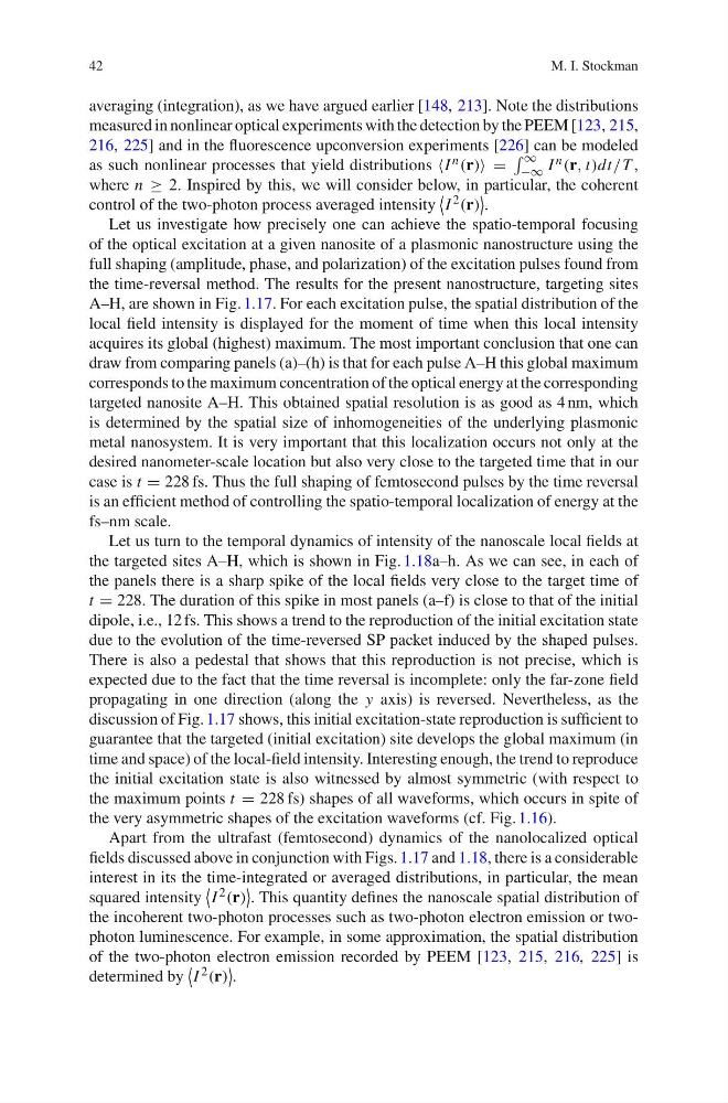
I 2 (r)
.
Let us investigate how precisely one can achieve the spatio-temporal focusing
of the optical excitation at a given nanosite of a plasmonic nanostructure using the
full shaping (amplitude, phase, and polarization) of the excitation pulses found from
the time-reversal method. The results for the present nanostructure, targeting sites
A–H, are shown in Fig. 1.17. For each excitation pulse, the spatial distribution of the
local field intensity is displayed for the moment of time when this local intensity
acquires its global (highest) maximum. The most important conclusion that one can
draw from comparing panels (a)–(h) is that for each pulse A–H this global maximum
corresponds to the maximum concentration of the optical energy at the corresponding
targeted nanosite A–H. This obtained spatial resolution is as good as 4 nm, which
is determined by the spatial size of inhomogeneities of the underlying plasmonic
metal nanosystem. It is very important that this localization occurs not only at the
desired nanometer-scale location but also very close to the targeted time that in our
case is t = 228 fs. Thus the full shaping of femtosecond pulses by the time reversal
is an efficient method of controlling the spatio-temporal localization of energy at the
fs–nm scale.
Let us turn to the temporal dynamics of intensity of the nanoscale local fields at
the targeted sites A–H, which is shown in Fig. 1.18a–h. As we can see, in each of
the panels there is a sharp spike of the local fields very close to the target time of
t = 228. The duration of this spike in most panels (a–f) is close to that of the initial
dipole, i.e., 12 fs. This shows a trend to the reproduction of the initial excitation state
due to the evolution of the time-reversed SP packet induced by the shaped pulses.
There is also a pedestal that shows that this reproduction is not precise, which is
expected due to the fact that the time reversal is incomplete: only the far-zone field
propagating in one direction (along the y axis) is reversed. Nevertheless, as the
discussion of Fig. 1.17 shows, this initial excitation-state reproduction is sufficient to
guarantee that the targeted (initial excitation) site develops the global maximum (in
time and space) of the local-field intensity. Interesting enough, the trend to reproduce
the initial excitation state is also witnessed by almost symmetric (with respect to
the maximum points t = 228 fs) shapes of all waveforms, which occurs in spite of
the very asymmetric shapes of the excitation waveforms (cf. Fig. 1.16).
Apart from the ultrafast (femtosecond) dynamics of the nanolocalized optical
fields discussed above in conjunction with Figs. 1.17 and 1.18, there is a considerable
interest in its the time-integrated or averaged distributions, in particular, the mean
squared intensity
I 2 (r)
. This quantity defines the nanoscale spatial distribution of
the incoherent two-photon processes such as two-photon electron emission or twophoton luminescence. For example, in some approximation, the spatial distribution
of the two-photon electron emission recorded by PEEM [123, 215, 216, 225] is
determined by
I 2 (r)
.
M. I. Stockman
averaging (integration), as we have argued earlier [148, 213]. Note the distributions
measured in nonlinear optical experiments with the detection by the PEEM [123, 215,
216, 225] and in the fluorescence upconversion experiments [226] can be modeled
as such nonlinear processes that yield distributions I n (r) =
∞
−∞ I n (r, t)dt/T ,
where n ≥ 2. Inspired by this, we will consider below, in particular, the coherent
control of the two-photon process averaged intensity
I 2 (r)
.
Let us investigate how precisely one can achieve the spatio-temporal focusing
of the optical excitation at a given nanosite of a plasmonic nanostructure using the
full shaping (amplitude, phase, and polarization) of the excitation pulses found from
the time-reversal method. The results for the present nanostructure, targeting sites
A–H, are shown in Fig. 1.17. For each excitation pulse, the spatial distribution of the
local field intensity is displayed for the moment of time when this local intensity
acquires its global (highest) maximum. The most important conclusion that one can
draw from comparing panels (a)–(h) is that for each pulse A–H this global maximum
corresponds to the maximum concentration of the optical energy at the corresponding
targeted nanosite A–H. This obtained spatial resolution is as good as 4 nm, which
is determined by the spatial size of inhomogeneities of the underlying plasmonic
metal nanosystem. It is very important that this localization occurs not only at the
desired nanometer-scale location but also very close to the targeted time that in our
case is t = 228 fs. Thus the full shaping of femtosecond pulses by the time reversal
is an efficient method of controlling the spatio-temporal localization of energy at the
fs–nm scale.
Let us turn to the temporal dynamics of intensity of the nanoscale local fields at
the targeted sites A–H, which is shown in Fig. 1.18a–h. As we can see, in each of
the panels there is a sharp spike of the local fields very close to the target time of
t = 228. The duration of this spike in most panels (a–f) is close to that of the initial
dipole, i.e., 12 fs. This shows a trend to the reproduction of the initial excitation state
due to the evolution of the time-reversed SP packet induced by the shaped pulses.
There is also a pedestal that shows that this reproduction is not precise, which is
expected due to the fact that the time reversal is incomplete: only the far-zone field
propagating in one direction (along the y axis) is reversed. Nevertheless, as the
discussion of Fig. 1.17 shows, this initial excitation-state reproduction is sufficient to
guarantee that the targeted (initial excitation) site develops the global maximum (in
time and space) of the local-field intensity. Interesting enough, the trend to reproduce
the initial excitation state is also witnessed by almost symmetric (with respect to
the maximum points t = 228 fs) shapes of all waveforms, which occurs in spite of
the very asymmetric shapes of the excitation waveforms (cf. Fig. 1.16).
Apart from the ultrafast (femtosecond) dynamics of the nanolocalized optical
fields discussed above in conjunction with Figs. 1.17 and 1.18, there is a considerable
interest in its the time-integrated or averaged distributions, in particular, the mean
squared intensity
I 2 (r)
. This quantity defines the nanoscale spatial distribution of
the incoherent two-photon processes such as two-photon electron emission or twophoton luminescence. For example, in some approximation, the spatial distribution
of the two-photon electron emission recorded by PEEM [123, 215, 216, 225] is
determined by
I 2 (r)
.