

1 Nanoplasmonics: From Present into Future
39
0
10
20
30
0
A
B
C
D
E
F
G
H
10
20
30 x (nm)
z (nm)
0
1
ε
t
228 fs
0
E z
E x
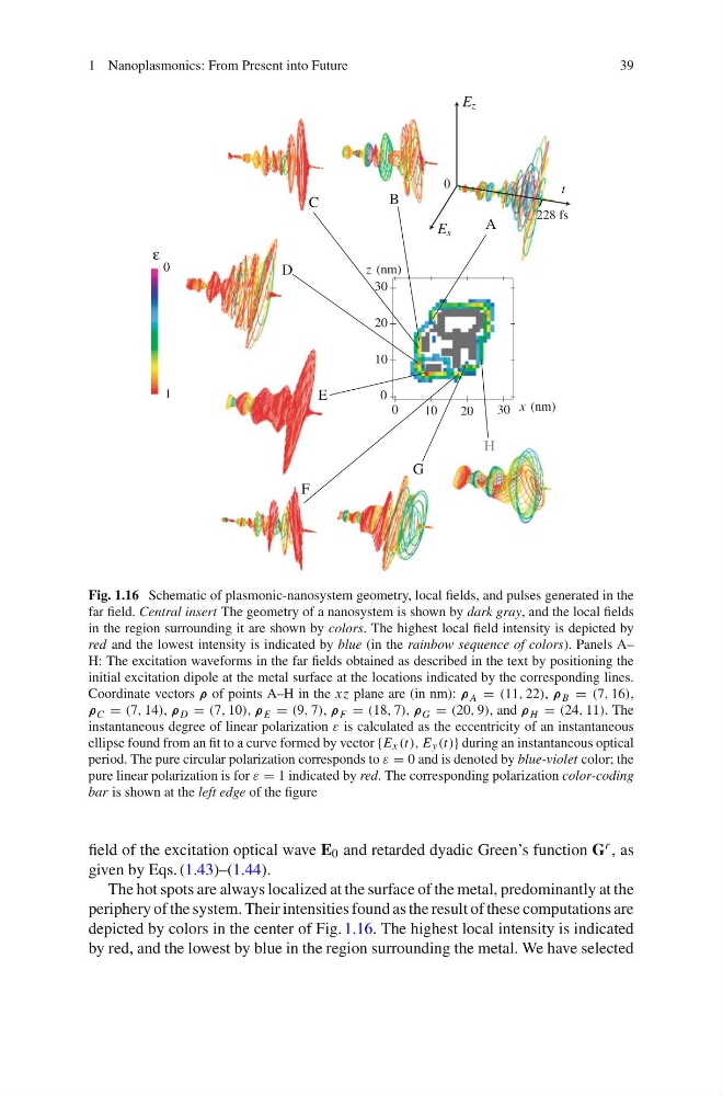
Fig. 1.16 Schematic of plasmonic-nanosystem geometry, local fields, and pulses generated in the
far field. Central insert The geometry of a nanosystem is shown by dark gray, and the local fields
in the region surrounding it are shown by colors. The highest local field intensity is depicted by
red and the lowest intensity is indicated by blue (in the rainbow sequence of colors). Panels A–
H: The excitation waveforms in the far fields obtained as described in the text by positioning the
initial excitation dipole at the metal surface at the locations indicated by the corresponding lines.
Coordinate vectors ρ of points A–H in the xz plane are (in nm): ρ A = (11, 22), ρ B = (7, 16),
ρ C = (7, 14), ρ D = (7, 10), ρ E = (9, 7), ρ F = (18, 7), ρ G = (20, 9), and ρ H = (24, 11). The
instantaneous degree of linear polarization ε is calculated as the eccentricity of an instantaneous
ellipse found from an fit to a curve formed by vector {E x (t), E y (t)} during an instantaneous optical
period. The pure circular polarization corresponds to ε = 0 and is denoted by blue-violet color; the
pure linear polarization is for ε = 1 indicated by red. The corresponding polarization color-coding
bar is shown at the left edge of the figure
field of the excitation optical wave E 0 and retarded dyadic Green’s function G r , as
given by Eqs. (1.43)–(1.44).
The hot spots are always localized at the surface of the metal, predominantly at the
periphery of the system. Their intensities found as the result of these computations are
depicted by colors in the center of Fig. 1.16. The highest local intensity is indicated
by red, and the lowest by blue in the region surrounding the metal. We have selected
39
0
10
20
30
0
A
B
C
D
E
F
G
H
10
20
30 x (nm)
z (nm)
0
1
ε
t
228 fs
0
E z
E x
Fig. 1.16 Schematic of plasmonic-nanosystem geometry, local fields, and pulses generated in the
far field. Central insert The geometry of a nanosystem is shown by dark gray, and the local fields
in the region surrounding it are shown by colors. The highest local field intensity is depicted by
red and the lowest intensity is indicated by blue (in the rainbow sequence of colors). Panels A–
H: The excitation waveforms in the far fields obtained as described in the text by positioning the
initial excitation dipole at the metal surface at the locations indicated by the corresponding lines.
Coordinate vectors ρ of points A–H in the xz plane are (in nm): ρ A = (11, 22), ρ B = (7, 16),
ρ C = (7, 14), ρ D = (7, 10), ρ E = (9, 7), ρ F = (18, 7), ρ G = (20, 9), and ρ H = (24, 11). The
instantaneous degree of linear polarization ε is calculated as the eccentricity of an instantaneous
ellipse found from an fit to a curve formed by vector {E x (t), E y (t)} during an instantaneous optical
period. The pure circular polarization corresponds to ε = 0 and is denoted by blue-violet color; the
pure linear polarization is for ε = 1 indicated by red. The corresponding polarization color-coding
bar is shown at the left edge of the figure
field of the excitation optical wave E 0 and retarded dyadic Green’s function G r , as
given by Eqs. (1.43)–(1.44).
The hot spots are always localized at the surface of the metal, predominantly at the
periphery of the system. Their intensities found as the result of these computations are
depicted by colors in the center of Fig. 1.16. The highest local intensity is indicated
by red, and the lowest by blue in the region surrounding the metal. We have selected