

176
K. M. Sørensen et al.
procedure is continued as long as the RMSEP (on the independent test set) decreases
by the introduction of a new variable. The result of this procedure is a set of variables
that represent the best combination in the spectral region, when optimizing for model
performance. However, it should be noted that the variable set found may not be the
absolute best one when compared to more sophisticated variable selection methods
due to the buildup nature of FSS. Like the VIP method, the FSS is based on regression
against y and it is thus important to use a test set, when evaluating the selection of
new variables. An evaluation procedure based on cross-validation only will often
lead to severe overfitting.
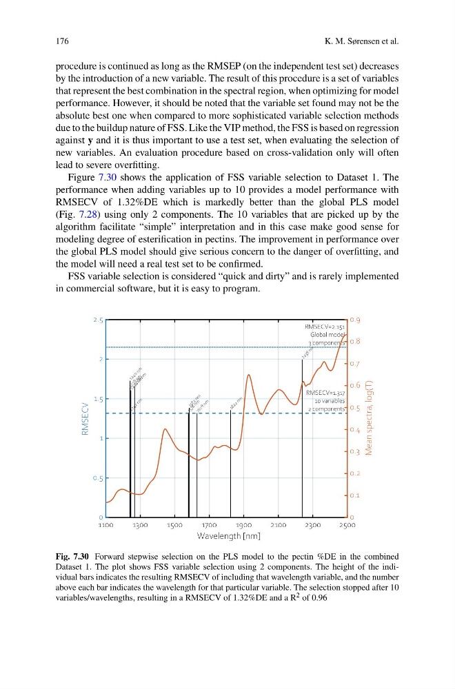
Figure 7.30 shows the application of FSS variable selection to Dataset 1. The
performance when adding variables up to 10 provides a model performance with
RMSECV of 1.32%DE which is markedly better than the global PLS model
(Fig. 7.28) using only 2 components. The 10 variables that are picked up by the
algorithm facilitate “simple” interpretation and in this case make good sense for
modeling degree of esterification in pectins. The improvement in performance over
the global PLS model should give serious concern to the danger of overfitting, and
the model will need a real test set to be confirmed.
FSS variable selection is considered “quick and dirty” and is rarely implemented
in commercial software, but it is easy to program.
1100
1300
1500
1700
1900
2100
2300
2500
Wavelength [nm]
0
0.5
1
1.5
2
2.5
RMSECV
0
0.1
0.2
0.3
0.4
0.5
0.6
0.7
0.8
0.9
Mean spectra, log(T)
2 2 3 8 n m
1 2 4 0 n m
1 2 6 6 n m
1 2 3 8 n m
1 2 4 4 n m
1 5 8 2
n m
1 8 2 2
n m
1 2 4 2
n m
1 5 7 8 n m
1 6 2 8 n m
RMSECV=1.317
10 variables
2 components
RMSECV=2.151
Global model
3 components
Fig. 7.30 Forward stepwise selection on the PLS model to the pectin %DE in the combined
Dataset 1. The plot shows FSS variable selection using 2 components. The height of the individual bars indicates the resulting RMSECV of including that wavelength variable, and the number
above each bar indicates the wavelength for that particular variable. The selection stopped after 10
variables/wavelengths, resulting in a RMSECV of 1.32%DE and a R 2 of 0.96
K. M. Sørensen et al.
procedure is continued as long as the RMSEP (on the independent test set) decreases
by the introduction of a new variable. The result of this procedure is a set of variables
that represent the best combination in the spectral region, when optimizing for model
performance. However, it should be noted that the variable set found may not be the
absolute best one when compared to more sophisticated variable selection methods
due to the buildup nature of FSS. Like the VIP method, the FSS is based on regression
against y and it is thus important to use a test set, when evaluating the selection of
new variables. An evaluation procedure based on cross-validation only will often
lead to severe overfitting.
Figure 7.30 shows the application of FSS variable selection to Dataset 1. The
performance when adding variables up to 10 provides a model performance with
RMSECV of 1.32%DE which is markedly better than the global PLS model
(Fig. 7.28) using only 2 components. The 10 variables that are picked up by the
algorithm facilitate “simple” interpretation and in this case make good sense for
modeling degree of esterification in pectins. The improvement in performance over
the global PLS model should give serious concern to the danger of overfitting, and
the model will need a real test set to be confirmed.
FSS variable selection is considered “quick and dirty” and is rarely implemented
in commercial software, but it is easy to program.
1100
1300
1500
1700
1900
2100
2300
2500
Wavelength [nm]
0
0.5
1
1.5
2
2.5
RMSECV
0
0.1
0.2
0.3
0.4
0.5
0.6
0.7
0.8
0.9
Mean spectra, log(T)
2 2 3 8 n m
1 2 4 0 n m
1 2 6 6 n m
1 2 3 8 n m
1 2 4 4 n m
1 5 8 2
n m
1 8 2 2
n m
1 2 4 2
n m
1 5 7 8 n m
1 6 2 8 n m
RMSECV=1.317
10 variables
2 components
RMSECV=2.151
Global model
3 components
Fig. 7.30 Forward stepwise selection on the PLS model to the pectin %DE in the combined
Dataset 1. The plot shows FSS variable selection using 2 components. The height of the individual bars indicates the resulting RMSECV of including that wavelength variable, and the number
above each bar indicates the wavelength for that particular variable. The selection stopped after 10
variables/wavelengths, resulting in a RMSECV of 1.32%DE and a R 2 of 0.96