

5 Introduction to Quantum Vibrational Spectroscopy
97
H = −
1
2
i
1
m i
∂
2
∂q
2
i
+
1
2
i
m i ω
2
0i q
2
i +
i≤j≤k
k ijk q i q j q k +
i≤j≤k≤l
k ijkl q i q j q k q l + · · ·
(5.1)
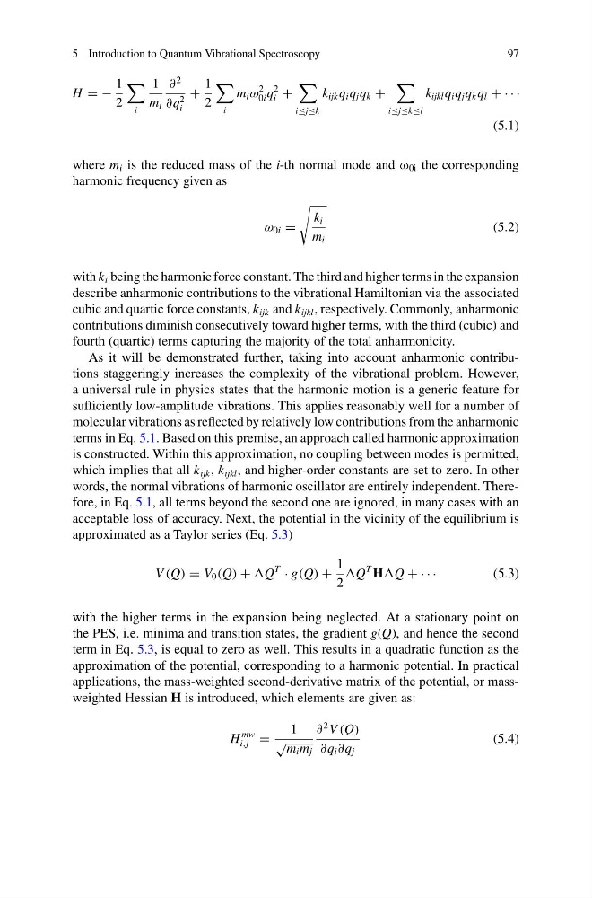
where m i is the reduced mass of the i-th normal mode and ω 0i the corresponding
harmonic frequency given as
ω 0i =
k i
m i
(5.2)
with k i being the harmonic force constant. The third and higher terms in the expansion
describe anharmonic contributions to the vibrational Hamiltonian via the associated
cubic and quartic force constants, k ijk and k ijkl , respectively. Commonly, anharmonic
contributions diminish consecutively toward higher terms, with the third (cubic) and
fourth (quartic) terms capturing the majority of the total anharmonicity.
As it will be demonstrated further, taking into account anharmonic contributions staggeringly increases the complexity of the vibrational problem. However,
a universal rule in physics states that the harmonic motion is a generic feature for
sufficiently low-amplitude vibrations. This applies reasonably well for a number of
molecular vibrations as reflected by relatively low contributions from the anharmonic
terms in Eq. 5.1. Based on this premise, an approach called harmonic approximation
is constructed. Within this approximation, no coupling between modes is permitted,
which implies that all k ijk , k ijkl , and higher-order constants are set to zero. In other
words, the normal vibrations of harmonic oscillator are entirely independent. Therefore, in Eq. 5.1, all terms beyond the second one are ignored, in many cases with an
acceptable loss of accuracy. Next, the potential in the vicinity of the equilibrium is
approximated as a Taylor series (Eq. 5.3)
V (Q) = V 0 (Q) + Q
T
· g(Q) +
1
2
Q
T HQ + · · ·
(5.3)
with the higher terms in the expansion being neglected. At a stationary point on
the PES, i.e. minima and transition states, the gradient g(Q), and hence the second
term in Eq. 5.3, is equal to zero as well. This results in a quadratic function as the
approximation of the potential, corresponding to a harmonic potential. In practical
applications, the mass-weighted second-derivative matrix of the potential, or massweighted Hessian H is introduced, which elements are given as:
H
mw
i,j =
1
√
m i m j
∂
2 V (Q)
∂q i ∂q j
(5.4)
97
H = −
1
2
i
1
m i
∂
2
∂q
2
i
+
1
2
i
m i ω
2
0i q
2
i +
i≤j≤k
k ijk q i q j q k +
i≤j≤k≤l
k ijkl q i q j q k q l + · · ·
(5.1)
where m i is the reduced mass of the i-th normal mode and ω 0i the corresponding
harmonic frequency given as
ω 0i =
k i
m i
(5.2)
with k i being the harmonic force constant. The third and higher terms in the expansion
describe anharmonic contributions to the vibrational Hamiltonian via the associated
cubic and quartic force constants, k ijk and k ijkl , respectively. Commonly, anharmonic
contributions diminish consecutively toward higher terms, with the third (cubic) and
fourth (quartic) terms capturing the majority of the total anharmonicity.
As it will be demonstrated further, taking into account anharmonic contributions staggeringly increases the complexity of the vibrational problem. However,
a universal rule in physics states that the harmonic motion is a generic feature for
sufficiently low-amplitude vibrations. This applies reasonably well for a number of
molecular vibrations as reflected by relatively low contributions from the anharmonic
terms in Eq. 5.1. Based on this premise, an approach called harmonic approximation
is constructed. Within this approximation, no coupling between modes is permitted,
which implies that all k ijk , k ijkl , and higher-order constants are set to zero. In other
words, the normal vibrations of harmonic oscillator are entirely independent. Therefore, in Eq. 5.1, all terms beyond the second one are ignored, in many cases with an
acceptable loss of accuracy. Next, the potential in the vicinity of the equilibrium is
approximated as a Taylor series (Eq. 5.3)
V (Q) = V 0 (Q) + Q
T
· g(Q) +
1
2
Q
T HQ + · · ·
(5.3)
with the higher terms in the expansion being neglected. At a stationary point on
the PES, i.e. minima and transition states, the gradient g(Q), and hence the second
term in Eq. 5.3, is equal to zero as well. This results in a quadratic function as the
approximation of the potential, corresponding to a harmonic potential. In practical
applications, the mass-weighted second-derivative matrix of the potential, or massweighted Hessian H is introduced, which elements are given as:
H
mw
i,j =
1
√
m i m j
∂
2 V (Q)
∂q i ∂q j
(5.4)