

26
P. K. Suresh
inflationary era and becomes zero at the end of the inflation stage. By considering
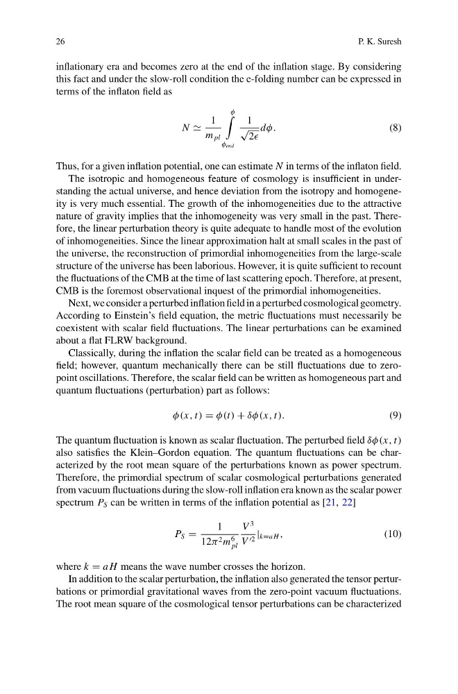
this fact and under the slow-roll condition the e-folding number can be expressed in
terms of the inflaton field as
N
1
m pl
φ
φ end
1
√
2
dφ.
(8)
Thus, for a given inflation potential, one can estimate N in terms of the inflaton field.
The isotropic and homogeneous feature of cosmology is insufficient in understanding the actual universe, and hence deviation from the isotropy and homogeneity is very much essential. The growth of the inhomogeneities due to the attractive
nature of gravity implies that the inhomogeneity was very small in the past. Therefore, the linear perturbation theory is quite adequate to handle most of the evolution
of inhomogeneities. Since the linear approximation halt at small scales in the past of
the universe, the reconstruction of primordial inhomogeneities from the large-scale
structure of the universe has been laborious. However, it is quite sufficient to recount
the fluctuations of the CMB at the time of last scattering epoch. Therefore, at present,
CMB is the foremost observational inquest of the primordial inhomogeneities.
Next, we consider a perturbed inflation field in a perturbed cosmological geometry.
According to Einstein’s field equation, the metric fluctuations must necessarily be
coexistent with scalar field fluctuations. The linear perturbations can be examined
about a flat FLRW background.
Classically, during the inflation the scalar field can be treated as a homogeneous
field; however, quantum mechanically there can be still fluctuations due to zeropoint oscillations. Therefore, the scalar field can be written as homogeneous part and
quantum fluctuations (perturbation) part as follows:
φ(x, t) = φ(t) + δφ(x, t).
(9)
The quantum fluctuation is known as scalar fluctuation. The perturbed field δφ(x, t)
also satisfies the Klein–Gordon equation. The quantum fluctuations can be characterized by the root mean square of the perturbations known as power spectrum.
Therefore, the primordial spectrum of scalar cosmological perturbations generated
from vacuum fluctuations during the slow-roll inflation era known as the scalar power
spectrum P S can be written in terms of the inflation potential as [21, 22]
P S =
1
12π 2 m
6
pl
V
3
V 2 | k=a H ,
(10)
where k = a H means the wave number crosses the horizon.
In addition to the scalar perturbation, the inflation also generated the tensor perturbations or primordial gravitational waves from the zero-point vacuum fluctuations.
The root mean square of the cosmological tensor perturbations can be characterized
P. K. Suresh
inflationary era and becomes zero at the end of the inflation stage. By considering
this fact and under the slow-roll condition the e-folding number can be expressed in
terms of the inflaton field as
N
1
m pl
φ
φ end
1
√
2
dφ.
(8)
Thus, for a given inflation potential, one can estimate N in terms of the inflaton field.
The isotropic and homogeneous feature of cosmology is insufficient in understanding the actual universe, and hence deviation from the isotropy and homogeneity is very much essential. The growth of the inhomogeneities due to the attractive
nature of gravity implies that the inhomogeneity was very small in the past. Therefore, the linear perturbation theory is quite adequate to handle most of the evolution
of inhomogeneities. Since the linear approximation halt at small scales in the past of
the universe, the reconstruction of primordial inhomogeneities from the large-scale
structure of the universe has been laborious. However, it is quite sufficient to recount
the fluctuations of the CMB at the time of last scattering epoch. Therefore, at present,
CMB is the foremost observational inquest of the primordial inhomogeneities.
Next, we consider a perturbed inflation field in a perturbed cosmological geometry.
According to Einstein’s field equation, the metric fluctuations must necessarily be
coexistent with scalar field fluctuations. The linear perturbations can be examined
about a flat FLRW background.
Classically, during the inflation the scalar field can be treated as a homogeneous
field; however, quantum mechanically there can be still fluctuations due to zeropoint oscillations. Therefore, the scalar field can be written as homogeneous part and
quantum fluctuations (perturbation) part as follows:
φ(x, t) = φ(t) + δφ(x, t).
(9)
The quantum fluctuation is known as scalar fluctuation. The perturbed field δφ(x, t)
also satisfies the Klein–Gordon equation. The quantum fluctuations can be characterized by the root mean square of the perturbations known as power spectrum.
Therefore, the primordial spectrum of scalar cosmological perturbations generated
from vacuum fluctuations during the slow-roll inflation era known as the scalar power
spectrum P S can be written in terms of the inflation potential as [21, 22]
P S =
1
12π 2 m
6
pl
V
3
V 2 | k=a H ,
(10)
where k = a H means the wave number crosses the horizon.
In addition to the scalar perturbation, the inflation also generated the tensor perturbations or primordial gravitational waves from the zero-point vacuum fluctuations.
The root mean square of the cosmological tensor perturbations can be characterized