

4.9 About Formation of Annular Speckle-Interferograms …
355
using this model are in good agreement with the data of the experimental studies of
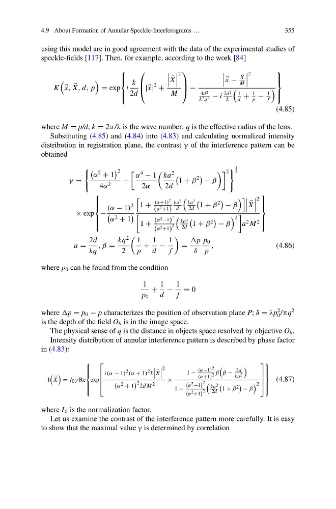
speckle-fields [117]. Then, for example, according to the work [84]
K
x,
X , d, p
= exp
⎧
⎪ ⎨
⎪ ⎩
i
k
2d
⎛
⎜
⎝ | x|
2 +
X
2
M
⎞
⎟
⎠ −
x −
X
M
2
4d 2
k 2 q 2 − i
2d 2
k
1
d
+
1
p
−
1
f
⎫
⎪ ⎬
⎪ ⎭
(4.85)
where M = p/d, k = 2π /λ is the wave number; q is the effective radius of the lens.
Substituting (4.85) and (4.84) into (4.83) and calculating normalized intensity
distribution in registration plane, the contrast γ of the interference pattern can be
obtained
γ =
α
2
+ 1
2
4α 2
+
α
4
− 1
2α
ka
2
2d
1 + β
2
− β
2 1
2
× exp
⎧
⎪ ⎪ ⎨
⎪ ⎪ ⎩
−
(α − 1)
2
α 2 + 1
1 +
(α+1)
2
(α
2 +1)
ka
2
d
ka
2
2d
1 + β
2
− β
X
2
1 + (α
2 −1)
2
(α
2 +1)
2
ka 2
2d
1 + β 2
− β
2
a 2 M 2
⎫
⎪ ⎪ ⎬
⎪ ⎪ ⎭
a =
2d
kq
, β =
kq
2
2
1
p
+
1
d
−
1
f
=
p
δ
p 0
p
,
(4.86)
where p 0 can be found from the condition
1
p 0
+
1
d
−
1
f
= 0
where p = p 0 − p characterizes the position of observation plane P; δ = λp
2
0 /πq
2
is the depth of the field O b is in the image space.
The physical sense of q is the distance in objects space resolved by objective O b .
Intensity distribution of annular interference pattern is described by phase factor
in (4.83):
I
X
= I 0 γ Re
⎧
⎪ ⎪ ⎪ ⎨
⎪ ⎪ ⎪ ⎩
exp
⎡
⎢
⎢
⎢
⎣
i(α − 1) 2 (α + 1) 2 k
X
2
α 2 + 1
2 2d M 2
×
1 −
(α−1) 2
(α+1) 2 β
β − 2d
ka 2
1 −
α 2 −1
2
α 2 +1
2
ka 2
2d
1 + β 2
− β
2
⎤
⎥
⎥
⎥
⎦
⎫
⎪ ⎪ ⎪ ⎬
⎪ ⎪ ⎪ ⎭
(4.87)
where I 0 is the normalization factor.
Let us examine the contrast of the interference pattern more carefully. It is easy
to show that the maximal value γ is determined by correlation
355
using this model are in good agreement with the data of the experimental studies of
speckle-fields [117]. Then, for example, according to the work [84]
K
x,
X , d, p
= exp
⎧
⎪ ⎨
⎪ ⎩
i
k
2d
⎛
⎜
⎝ | x|
2 +
X
2
M
⎞
⎟
⎠ −
x −
X
M
2
4d 2
k 2 q 2 − i
2d 2
k
1
d
+
1
p
−
1
f
⎫
⎪ ⎬
⎪ ⎭
(4.85)
where M = p/d, k = 2π /λ is the wave number; q is the effective radius of the lens.
Substituting (4.85) and (4.84) into (4.83) and calculating normalized intensity
distribution in registration plane, the contrast γ of the interference pattern can be
obtained
γ =
α
2
+ 1
2
4α 2
+
α
4
− 1
2α
ka
2
2d
1 + β
2
− β
2 1
2
× exp
⎧
⎪ ⎪ ⎨
⎪ ⎪ ⎩
−
(α − 1)
2
α 2 + 1
1 +
(α+1)
2
(α
2 +1)
ka
2
d
ka
2
2d
1 + β
2
− β
X
2
1 + (α
2 −1)
2
(α
2 +1)
2
ka 2
2d
1 + β 2
− β
2
a 2 M 2
⎫
⎪ ⎪ ⎬
⎪ ⎪ ⎭
a =
2d
kq
, β =
kq
2
2
1
p
+
1
d
−
1
f
=
p
δ
p 0
p
,
(4.86)
where p 0 can be found from the condition
1
p 0
+
1
d
−
1
f
= 0
where p = p 0 − p characterizes the position of observation plane P; δ = λp
2
0 /πq
2
is the depth of the field O b is in the image space.
The physical sense of q is the distance in objects space resolved by objective O b .
Intensity distribution of annular interference pattern is described by phase factor
in (4.83):
I
X
= I 0 γ Re
⎧
⎪ ⎪ ⎪ ⎨
⎪ ⎪ ⎪ ⎩
exp
⎡
⎢
⎢
⎢
⎣
i(α − 1) 2 (α + 1) 2 k
X
2
α 2 + 1
2 2d M 2
×
1 −
(α−1) 2
(α+1) 2 β
β − 2d
ka 2
1 −
α 2 −1
2
α 2 +1
2
ka 2
2d
1 + β 2
− β
2
⎤
⎥
⎥
⎥
⎦
⎫
⎪ ⎪ ⎪ ⎬
⎪ ⎪ ⎪ ⎭
(4.87)
where I 0 is the normalization factor.
Let us examine the contrast of the interference pattern more carefully. It is easy
to show that the maximal value γ is determined by correlation