

2.2 Holographic Study of Structural and Functional Characteristics …
115
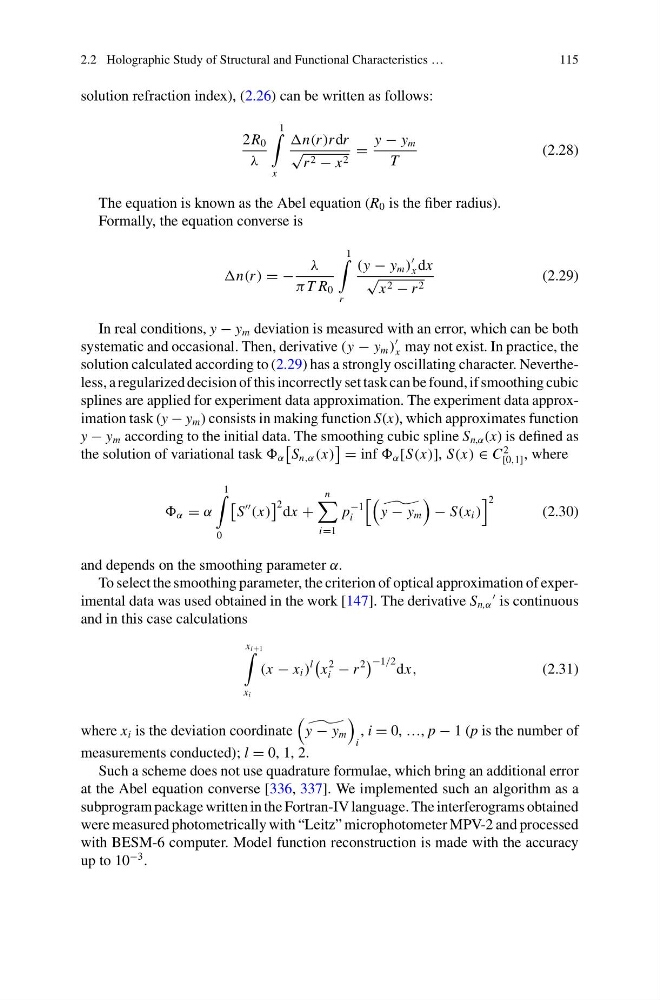
solution refraction index), (2.26) can be written as follows:
2R 0
λ
1
x
n(r )r dr
√
r 2 − x 2
=
y − y m
T
(2.28)
The equation is known as the Abel equation (R 0 is the fiber radius).
Formally, the equation converse is
n(r ) = −
λ
π T R 0
1
r
(y − y m )
x dx
√
x 2 − r 2
(2.29)
In real conditions, y − y m deviation is measured with an error, which can be both
systematic and occasional. Then, derivative (y − y m )
x may not exist. In practice, the
solution calculated according to (2.29) has a strongly oscillating character. Nevertheless, a regularized decision of this incorrectly set task can be found, if smoothing cubic
splines are applied for experiment data approximation. The experiment data approximation task (y − y m ) consists in making function S(x), which approximates function
y − y m according to the initial data. The smoothing cubic spline S n,α (x) is defined as
the solution of variational task α
S n,α (x)
= inf α [S(x)], S(x) ∈ C
2
[0,1] , where
α = α
1
0
S
(x)
2 dx +
n
i=1
p
−1
i
y − y m
− S(x i )
2
(2.30)
and depends on the smoothing parameter α.
To select the smoothing parameter, the criterion of optical approximation of experimental data was used obtained in the work [147]. The derivative S n,α
is continuous
and in this case calculations
x i+1
x i
(x − x i )
l
x
2
i − r
2
−1/2 dx,
(2.31)
where x i is the deviation coordinate
y − y m
i
, i = 0, …, p − 1 (p is the number of
measurements conducted); l = 0, 1, 2.
Such a scheme does not use quadrature formulae, which bring an additional error
at the Abel equation converse [336, 337]. We implemented such an algorithm as a
subprogram package written in the Fortran-IV language. The interferograms obtained
were measured photometrically with “Leitz” microphotometer MPV-2 and processed
with BESM-6 computer. Model function reconstruction is made with the accuracy
up to 10
−3 .
115
solution refraction index), (2.26) can be written as follows:
2R 0
λ
1
x
n(r )r dr
√
r 2 − x 2
=
y − y m
T
(2.28)
The equation is known as the Abel equation (R 0 is the fiber radius).
Formally, the equation converse is
n(r ) = −
λ
π T R 0
1
r
(y − y m )
x dx
√
x 2 − r 2
(2.29)
In real conditions, y − y m deviation is measured with an error, which can be both
systematic and occasional. Then, derivative (y − y m )
x may not exist. In practice, the
solution calculated according to (2.29) has a strongly oscillating character. Nevertheless, a regularized decision of this incorrectly set task can be found, if smoothing cubic
splines are applied for experiment data approximation. The experiment data approximation task (y − y m ) consists in making function S(x), which approximates function
y − y m according to the initial data. The smoothing cubic spline S n,α (x) is defined as
the solution of variational task α
S n,α (x)
= inf α [S(x)], S(x) ∈ C
2
[0,1] , where
α = α
1
0
S
(x)
2 dx +
n
i=1
p
−1
i
y − y m
− S(x i )
2
(2.30)
and depends on the smoothing parameter α.
To select the smoothing parameter, the criterion of optical approximation of experimental data was used obtained in the work [147]. The derivative S n,α
is continuous
and in this case calculations
x i+1
x i
(x − x i )
l
x
2
i − r
2
−1/2 dx,
(2.31)
where x i is the deviation coordinate
y − y m
i
, i = 0, …, p − 1 (p is the number of
measurements conducted); l = 0, 1, 2.
Such a scheme does not use quadrature formulae, which bring an additional error
at the Abel equation converse [336, 337]. We implemented such an algorithm as a
subprogram package written in the Fortran-IV language. The interferograms obtained
were measured photometrically with “Leitz” microphotometer MPV-2 and processed
with BESM-6 computer. Model function reconstruction is made with the accuracy
up to 10
−3 .