

2.3 Implementation of Numerical Solution
31
velocity component between two grid points, and the establishment of the relationship
between pressure gradient and velocity creates conditions for the iterative solution.
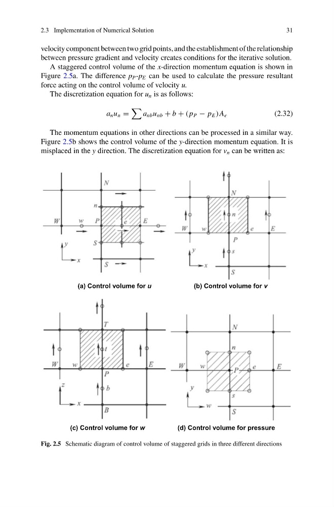
A staggered control volume of the x-direction momentum equation is shown in
Figure 2.5a. The difference p P -p E can be used to calculate the pressure resultant
force acting on the control volume of velocity u.
The discretization equation for u n is as follows:
a n u n =
a nb u nb + b + ( p P − p E )A e
(2.32)
The momentum equations in other directions can be processed in a similar way.
Figure 2.5b shows the control volume of the y-direction momentum equation. It is
misplaced in the y direction. The discretization equation for v n can be written as:
(a) Control volume for u
(b) Control volume for v
(c) Control volume for w
(d) Control volume for pressure
Fig. 2.5 Schematic diagram of control volume of staggered grids in three different directions
31
velocity component between two grid points, and the establishment of the relationship
between pressure gradient and velocity creates conditions for the iterative solution.
A staggered control volume of the x-direction momentum equation is shown in
Figure 2.5a. The difference p P -p E can be used to calculate the pressure resultant
force acting on the control volume of velocity u.
The discretization equation for u n is as follows:
a n u n =
a nb u nb + b + ( p P − p E )A e
(2.32)
The momentum equations in other directions can be processed in a similar way.
Figure 2.5b shows the control volume of the y-direction momentum equation. It is
misplaced in the y direction. The discretization equation for v n can be written as:
(a) Control volume for u
(b) Control volume for v
(c) Control volume for w
(d) Control volume for pressure
Fig. 2.5 Schematic diagram of control volume of staggered grids in three different directions