

76
3 Modeling Composite Structures
-20000
-10000
0
10000
20000
30000
40000
0
10 20 30 40 50 60 70 80 90 100
R
Freq(MHz)
25
75
125
Host
-40000
-35000
-30000
-25000
-20000
-15000
-10000
-5000
0
5000
0
10 20 30 40 50 60 70 80 90 100
X
Freq(MHz)
25
75
125
Host
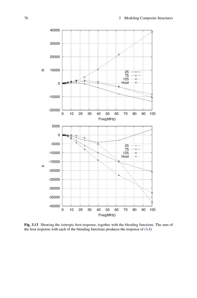
Fig. 3.13 Showing the isotropic host response, together with the blending functions. The sum of
the host response with each of the blending functions produces the response of (3.4)
3 Modeling Composite Structures
-20000
-10000
0
10000
20000
30000
40000
0
10 20 30 40 50 60 70 80 90 100
R
Freq(MHz)
25
75
125
Host
-40000
-35000
-30000
-25000
-20000
-15000
-10000
-5000
0
5000
0
10 20 30 40 50 60 70 80 90 100
X
Freq(MHz)
25
75
125
Host
Fig. 3.13 Showing the isotropic host response, together with the blending functions. The sum of
the host response with each of the blending functions produces the response of (3.4)