

2.6 Application to Aircraft Structures
47
0.1
1
10
-1 -0.8 -0.6 -0.4 -0.2 0 0.2 0.4 0.6 0.8 1
Scale (S)
Normalized anomalous conductivity
Convergence of estimates for cells 86 and 87
cell no. 86
cell no. 87
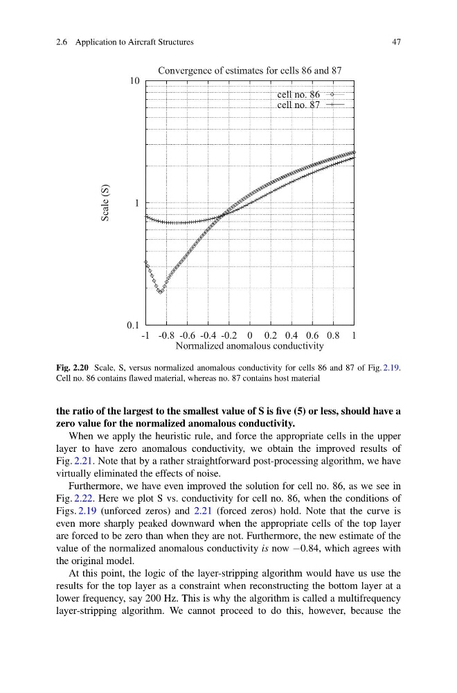
Fig. 2.20 Scale, S, versus normalized anomalous conductivity for cells 86 and 87 of Fig. 2.19.
Cell no. 86 contains flawed material, whereas no. 87 contains host material
the ratio of the largest to the smallest value of S is five (5) or less, should have a
zero value for the normalized anomalous conductivity.
When we apply the heuristic rule, and force the appropriate cells in the upper
layer to have zero anomalous conductivity, we obtain the improved results of
Fig. 2.21. Note that by a rather straightforward post-processing algorithm, we have
virtually eliminated the effects of noise.
Furthermore, we have even improved the solution for cell no. 86, as we see in
Fig. 2.22. Here we plot S vs. conductivity for cell no. 86, when the conditions of
Figs. 2.19 (unforced zeros) and 2.21 (forced zeros) hold. Note that the curve is
even more sharply peaked downward when the appropriate cells of the top layer
are forced to be zero than when they are not. Furthermore, the new estimate of the
value of the normalized anomalous conductivity is now −0.84, which agrees with
the original model.
At this point, the logic of the layer-stripping algorithm would have us use the
results for the top layer as a constraint when reconstructing the bottom layer at a
lower frequency, say 200 Hz. This is why the algorithm is called a multifrequency
layer-stripping algorithm. We cannot proceed to do this, however, because the
47
0.1
1
10
-1 -0.8 -0.6 -0.4 -0.2 0 0.2 0.4 0.6 0.8 1
Scale (S)
Normalized anomalous conductivity
Convergence of estimates for cells 86 and 87
cell no. 86
cell no. 87
Fig. 2.20 Scale, S, versus normalized anomalous conductivity for cells 86 and 87 of Fig. 2.19.
Cell no. 86 contains flawed material, whereas no. 87 contains host material
the ratio of the largest to the smallest value of S is five (5) or less, should have a
zero value for the normalized anomalous conductivity.
When we apply the heuristic rule, and force the appropriate cells in the upper
layer to have zero anomalous conductivity, we obtain the improved results of
Fig. 2.21. Note that by a rather straightforward post-processing algorithm, we have
virtually eliminated the effects of noise.
Furthermore, we have even improved the solution for cell no. 86, as we see in
Fig. 2.22. Here we plot S vs. conductivity for cell no. 86, when the conditions of
Figs. 2.19 (unforced zeros) and 2.21 (forced zeros) hold. Note that the curve is
even more sharply peaked downward when the appropriate cells of the top layer
are forced to be zero than when they are not. Furthermore, the new estimate of the
value of the normalized anomalous conductivity is now −0.84, which agrees with
the original model.
At this point, the logic of the layer-stripping algorithm would have us use the
results for the top layer as a constraint when reconstructing the bottom layer at a
lower frequency, say 200 Hz. This is why the algorithm is called a multifrequency
layer-stripping algorithm. We cannot proceed to do this, however, because the