

30
2 Voxel-Based Inversion Via Set-Theoretic Estimation
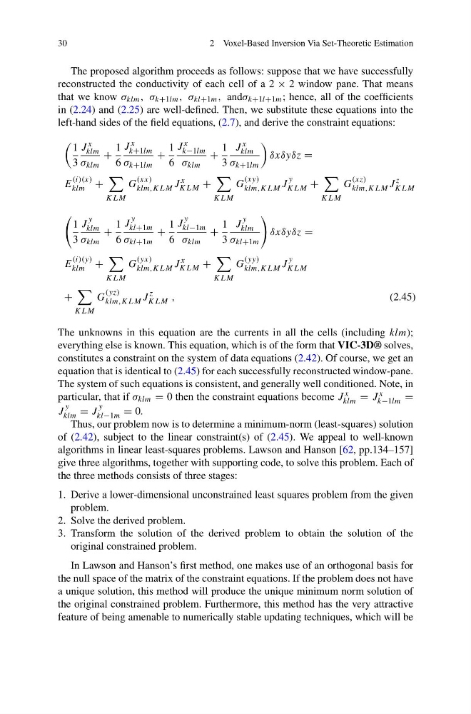
The proposed algorithm proceeds as follows: suppose that we have successfully
reconstructed the conductivity of each cell of a 2 × 2 window pane. That means
that we know σ klm , σ k+1lm , σ kl+1m , andσ k+1l+1m ; hence, all of the coefficients
in (2.24) and (2.25) are well-defined. Then, we substitute these equations into the
left-hand sides of the field equations, (2.7), and derive the constraint equations:
1
3
J x
klm
σ klm
+
1
6
J x
k+1lm
σ k+1lm
+
1
6
J x
k−1lm
σ klm
+
1
3
J x
klm
σ k+1lm
δxδyδz =
E
(i)(x)
klm +
KLM
G
(xx)
klm,KLM J
x
KLM +
KLM
G
(xy)
klm,KLM J
y
KLM +
KLM
G
(xz)
klm,KLM J
z
KLM
1
3
J
y
klm
σ klm
+
1
6
J
y
kl+1m
σ kl+1m
+
1
6
J
y
kl−1m
σ klm
+
1
3
J
y
klm
σ kl+1m
δxδyδz =
E
(i)(y)
klm +
KLM
G
(yx)
klm,KLM J
x
KLM +
KLM
G
(yy)
klm,KLM J
y
KLM
+
KLM
G
(yz)
klm,KLM J
z
KLM ,
(2.45)
The unknowns in this equation are the currents in all the cells (including klm);
everything else is known. This equation, which is of the form that VIC-3D® solves,
constitutes a constraint on the system of data equations (2.42). Of course, we get an
equation that is identical to (2.45) for each successfully reconstructed window-pane.
The system of such equations is consistent, and generally well conditioned. Note, in
particular, that if σ klm = 0 then the constraint equations become J x
klm = J x
k−1lm =
J
y
klm = J
y
kl−1m = 0.
Thus, our problem now is to determine a minimum-norm (least-squares) solution
of (2.42), subject to the linear constraint(s) of (2.45). We appeal to well-known
algorithms in linear least-squares problems. Lawson and Hanson [62, pp.134–157]
give three algorithms, together with supporting code, to solve this problem. Each of
the three methods consists of three stages:
1. Derive a lower-dimensional unconstrained least squares problem from the given
problem.
2. Solve the derived problem.
3. Transform the solution of the derived problem to obtain the solution of the
original constrained problem.
In Lawson and Hanson’s first method, one makes use of an orthogonal basis for
the null space of the matrix of the constraint equations. If the problem does not have
a unique solution, this method will produce the unique minimum norm solution of
the original constrained problem. Furthermore, this method has the very attractive
feature of being amenable to numerically stable updating techniques, which will be
2 Voxel-Based Inversion Via Set-Theoretic Estimation
The proposed algorithm proceeds as follows: suppose that we have successfully
reconstructed the conductivity of each cell of a 2 × 2 window pane. That means
that we know σ klm , σ k+1lm , σ kl+1m , andσ k+1l+1m ; hence, all of the coefficients
in (2.24) and (2.25) are well-defined. Then, we substitute these equations into the
left-hand sides of the field equations, (2.7), and derive the constraint equations:
1
3
J x
klm
σ klm
+
1
6
J x
k+1lm
σ k+1lm
+
1
6
J x
k−1lm
σ klm
+
1
3
J x
klm
σ k+1lm
δxδyδz =
E
(i)(x)
klm +
KLM
G
(xx)
klm,KLM J
x
KLM +
KLM
G
(xy)
klm,KLM J
y
KLM +
KLM
G
(xz)
klm,KLM J
z
KLM
1
3
J
y
klm
σ klm
+
1
6
J
y
kl+1m
σ kl+1m
+
1
6
J
y
kl−1m
σ klm
+
1
3
J
y
klm
σ kl+1m
δxδyδz =
E
(i)(y)
klm +
KLM
G
(yx)
klm,KLM J
x
KLM +
KLM
G
(yy)
klm,KLM J
y
KLM
+
KLM
G
(yz)
klm,KLM J
z
KLM ,
(2.45)
The unknowns in this equation are the currents in all the cells (including klm);
everything else is known. This equation, which is of the form that VIC-3D® solves,
constitutes a constraint on the system of data equations (2.42). Of course, we get an
equation that is identical to (2.45) for each successfully reconstructed window-pane.
The system of such equations is consistent, and generally well conditioned. Note, in
particular, that if σ klm = 0 then the constraint equations become J x
klm = J x
k−1lm =
J
y
klm = J
y
kl−1m = 0.
Thus, our problem now is to determine a minimum-norm (least-squares) solution
of (2.42), subject to the linear constraint(s) of (2.45). We appeal to well-known
algorithms in linear least-squares problems. Lawson and Hanson [62, pp.134–157]
give three algorithms, together with supporting code, to solve this problem. Each of
the three methods consists of three stages:
1. Derive a lower-dimensional unconstrained least squares problem from the given
problem.
2. Solve the derived problem.
3. Transform the solution of the derived problem to obtain the solution of the
original constrained problem.
In Lawson and Hanson’s first method, one makes use of an orthogonal basis for
the null space of the matrix of the constraint equations. If the problem does not have
a unique solution, this method will produce the unique minimum norm solution of
the original constrained problem. Furthermore, this method has the very attractive
feature of being amenable to numerically stable updating techniques, which will be