

12.8 Inverse Problems
339
of cos(φ) in (2) of the
σ = 2.205E6
Ti:
Crystallites (grains)
σ determined by
random distribution
text, using a uniform
distribution function.
a
:
Coil
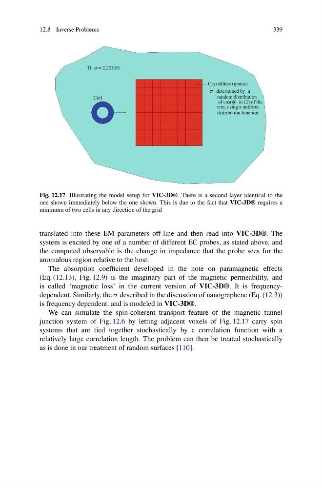
Fig. 12.17 Illustrating the model setup for VIC-3D®. There is a second layer identical to the
one shown immediately below the one shown. This is due to the fact that VIC-3D® requires a
minimum of two cells in any direction of the grid
translated into these EM parameters off-line and then read into VIC-3D®. The
system is excited by one of a number of different EC probes, as stated above, and
the computed observable is the change in impedance that the probe sees for the
anomalous region relative to the host.
The absorption coefficient developed in the note on paramagnetic effects
(Eq. (12.13), Fig. 12.9) is the imaginary part of the magnetic permeability, and
is called ‘magnetic loss’ in the current version of VIC-3D®. It is frequencydependent. Similarly, the σ described in the discussion of nanographene (Eq. (12.3))
is frequency dependent, and is modeled in VIC-3D®.
We can simulate the spin-coherent transport feature of the magnetic tunnel
junction system of Fig. 12.6 by letting adjacent voxels of Fig. 12.17 carry spin
systems that are tied together stochastically by a correlation function with a
relatively large correlation length. The problem can then be treated stochastically
as is done in our treatment of random surfaces [110].
339
of cos(φ) in (2) of the
σ = 2.205E6
Ti:
Crystallites (grains)
σ determined by
random distribution
text, using a uniform
distribution function.
a
:
Coil
Fig. 12.17 Illustrating the model setup for VIC-3D®. There is a second layer identical to the
one shown immediately below the one shown. This is due to the fact that VIC-3D® requires a
minimum of two cells in any direction of the grid
translated into these EM parameters off-line and then read into VIC-3D®. The
system is excited by one of a number of different EC probes, as stated above, and
the computed observable is the change in impedance that the probe sees for the
anomalous region relative to the host.
The absorption coefficient developed in the note on paramagnetic effects
(Eq. (12.13), Fig. 12.9) is the imaginary part of the magnetic permeability, and
is called ‘magnetic loss’ in the current version of VIC-3D®. It is frequencydependent. Similarly, the σ described in the discussion of nanographene (Eq. (12.3))
is frequency dependent, and is modeled in VIC-3D®.
We can simulate the spin-coherent transport feature of the magnetic tunnel
junction system of Fig. 12.6 by letting adjacent voxels of Fig. 12.17 carry spin
systems that are tied together stochastically by a correlation function with a
relatively large correlation length. The problem can then be treated stochastically
as is done in our treatment of random surfaces [110].