

10.10 Comments and Discussion
275
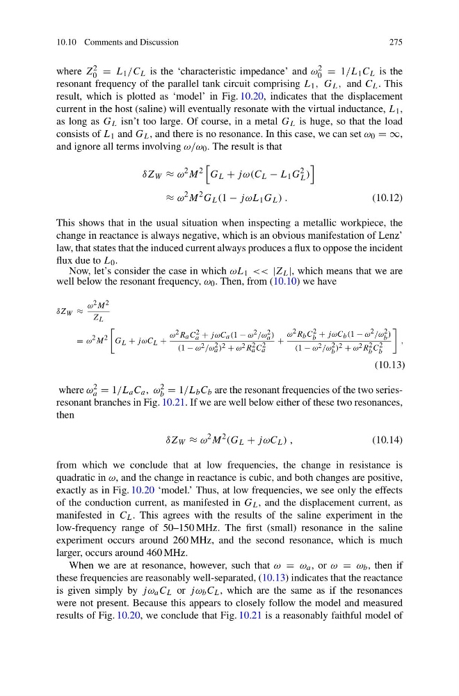
where Z 2
0 = L 1 /C L is the ‘characteristic impedance’ and ω 2
0 = 1/L 1 C L is the
resonant frequency of the parallel tank circuit comprising L 1 , G L , and C L . This
result, which is plotted as ‘model’ in Fig. 10.20, indicates that the displacement
current in the host (saline) will eventually resonate with the virtual inductance, L 1 ,
as long as G L isn’t too large. Of course, in a metal G L is huge, so that the load
consists of L 1 and G L , and there is no resonance. In this case, we can set ω 0 = ∞,
and ignore all terms involving ω/ω 0 . The result is that
δZ W ≈ ω
2 M
2
G L + jω(C L − L 1 G
2
L )
≈ ω
2 M
2 G L (1 − jωL 1 G L ) .
(10.12)
This shows that in the usual situation when inspecting a metallic workpiece, the
change in reactance is always negative, which is an obvious manifestation of Lenz’
law, that states that the induced current always produces a flux to oppose the incident
flux due to L 0 .
Now, let’s consider the case in which ωL 1 << |Z L |, which means that we are
well below the resonant frequency, ω 0 . Then, from (10.10) we have
δZ W ≈
ω 2 M 2
Z L
= ω 2 M 2
G L + jωC L +
ω 2 R a C 2
a + jωC a (1 − ω 2 /ω 2
a )
(1 − ω 2 /ω 2
a ) 2 + ω 2 R 2
a C 2
a
+
ω 2 R b C 2
b + jωC b (1 − ω 2 /ω 2
b )
(1 − ω 2 /ω 2
b ) 2 + ω 2 R 2
b C 2
b
,
(10.13)
where ω 2
a = 1/L a C a , ω 2
b = 1/L b C b are the resonant frequencies of the two seriesresonant branches in Fig. 10.21. If we are well below either of these two resonances,
then
δZ W ≈ ω
2 M
2 (G L + jωC L ) ,
(10.14)
from which we conclude that at low frequencies, the change in resistance is
quadratic in ω, and the change in reactance is cubic, and both changes are positive,
exactly as in Fig. 10.20 ‘model.’ Thus, at low frequencies, we see only the effects
of the conduction current, as manifested in G L , and the displacement current, as
manifested in C L . This agrees with the results of the saline experiment in the
low-frequency range of 50–150 MHz. The first (small) resonance in the saline
experiment occurs around 260 MHz, and the second resonance, which is much
larger, occurs around 460 MHz.
When we are at resonance, however, such that ω = ω a , or ω = ω b , then if
these frequencies are reasonably well-separated, (10.13) indicates that the reactance
is given simply by jω a C L or jω b C L , which are the same as if the resonances
were not present. Because this appears to closely follow the model and measured
results of Fig. 10.20, we conclude that Fig. 10.21 is a reasonably faithful model of
275
where Z 2
0 = L 1 /C L is the ‘characteristic impedance’ and ω 2
0 = 1/L 1 C L is the
resonant frequency of the parallel tank circuit comprising L 1 , G L , and C L . This
result, which is plotted as ‘model’ in Fig. 10.20, indicates that the displacement
current in the host (saline) will eventually resonate with the virtual inductance, L 1 ,
as long as G L isn’t too large. Of course, in a metal G L is huge, so that the load
consists of L 1 and G L , and there is no resonance. In this case, we can set ω 0 = ∞,
and ignore all terms involving ω/ω 0 . The result is that
δZ W ≈ ω
2 M
2
G L + jω(C L − L 1 G
2
L )
≈ ω
2 M
2 G L (1 − jωL 1 G L ) .
(10.12)
This shows that in the usual situation when inspecting a metallic workpiece, the
change in reactance is always negative, which is an obvious manifestation of Lenz’
law, that states that the induced current always produces a flux to oppose the incident
flux due to L 0 .
Now, let’s consider the case in which ωL 1 << |Z L |, which means that we are
well below the resonant frequency, ω 0 . Then, from (10.10) we have
δZ W ≈
ω 2 M 2
Z L
= ω 2 M 2
G L + jωC L +
ω 2 R a C 2
a + jωC a (1 − ω 2 /ω 2
a )
(1 − ω 2 /ω 2
a ) 2 + ω 2 R 2
a C 2
a
+
ω 2 R b C 2
b + jωC b (1 − ω 2 /ω 2
b )
(1 − ω 2 /ω 2
b ) 2 + ω 2 R 2
b C 2
b
,
(10.13)
where ω 2
a = 1/L a C a , ω 2
b = 1/L b C b are the resonant frequencies of the two seriesresonant branches in Fig. 10.21. If we are well below either of these two resonances,
then
δZ W ≈ ω
2 M
2 (G L + jωC L ) ,
(10.14)
from which we conclude that at low frequencies, the change in resistance is
quadratic in ω, and the change in reactance is cubic, and both changes are positive,
exactly as in Fig. 10.20 ‘model.’ Thus, at low frequencies, we see only the effects
of the conduction current, as manifested in G L , and the displacement current, as
manifested in C L . This agrees with the results of the saline experiment in the
low-frequency range of 50–150 MHz. The first (small) resonance in the saline
experiment occurs around 260 MHz, and the second resonance, which is much
larger, occurs around 460 MHz.
When we are at resonance, however, such that ω = ω a , or ω = ω b , then if
these frequencies are reasonably well-separated, (10.13) indicates that the reactance
is given simply by jω a C L or jω b C L , which are the same as if the resonances
were not present. Because this appears to closely follow the model and measured
results of Fig. 10.20, we conclude that Fig. 10.21 is a reasonably faithful model of