

9.9 A Five-Dimensional Inverse Problem
241
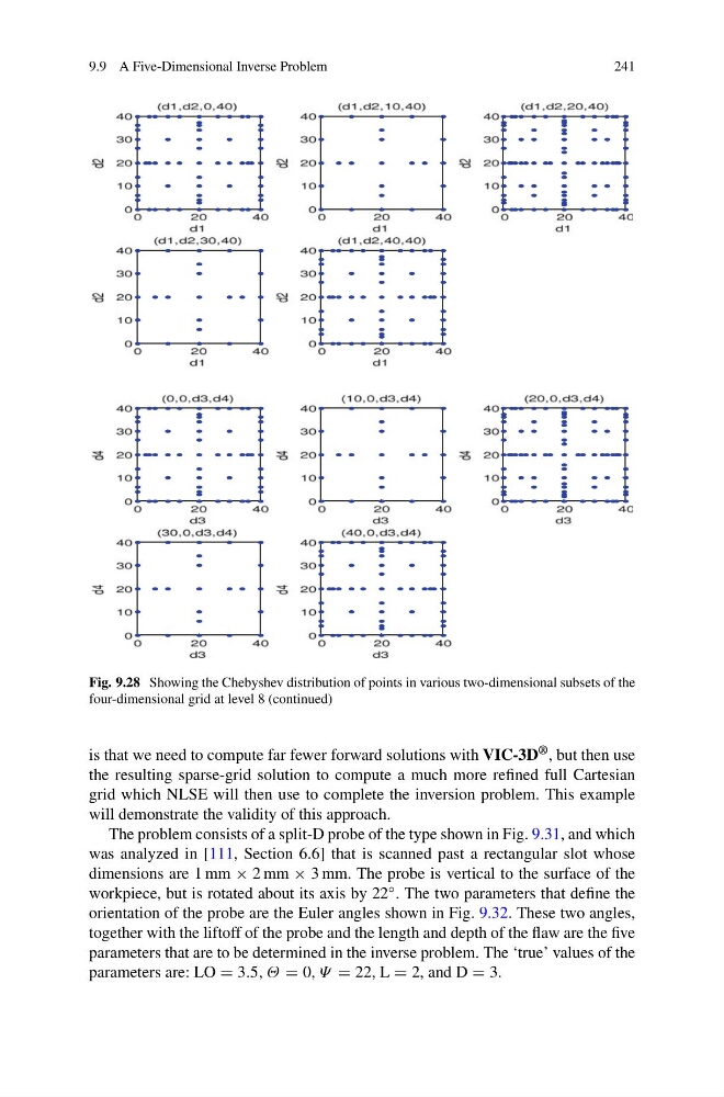
Fig. 9.28 Showing the Chebyshev distribution of points in various two-dimensional subsets of the
four-dimensional grid at level 8 (continued)
is that we need to compute far fewer forward solutions with VIC-3D ® , but then use
the resulting sparse-grid solution to compute a much more refined full Cartesian
grid which NLSE will then use to complete the inversion problem. This example
will demonstrate the validity of this approach.
The problem consists of a split-D probe of the type shown in Fig. 9.31, and which
was analyzed in [111, Section 6.6] that is scanned past a rectangular slot whose
dimensions are 1 mm × 2 mm × 3 mm. The probe is vertical to the surface of the
workpiece, but is rotated about its axis by 22 ◦ . The two parameters that define the
orientation of the probe are the Euler angles shown in Fig. 9.32. These two angles,
together with the liftoff of the probe and the length and depth of the flaw are the five
parameters that are to be determined in the inverse problem. The ‘true’ values of the
parameters are: LO = 3.5, Θ = 0, Ψ = 22, L = 2, and D = 3.
241
Fig. 9.28 Showing the Chebyshev distribution of points in various two-dimensional subsets of the
four-dimensional grid at level 8 (continued)
is that we need to compute far fewer forward solutions with VIC-3D ® , but then use
the resulting sparse-grid solution to compute a much more refined full Cartesian
grid which NLSE will then use to complete the inversion problem. This example
will demonstrate the validity of this approach.
The problem consists of a split-D probe of the type shown in Fig. 9.31, and which
was analyzed in [111, Section 6.6] that is scanned past a rectangular slot whose
dimensions are 1 mm × 2 mm × 3 mm. The probe is vertical to the surface of the
workpiece, but is rotated about its axis by 22 ◦ . The two parameters that define the
orientation of the probe are the Euler angles shown in Fig. 9.32. These two angles,
together with the liftoff of the probe and the length and depth of the flaw are the five
parameters that are to be determined in the inverse problem. The ‘true’ values of the
parameters are: LO = 3.5, Θ = 0, Ψ = 22, L = 2, and D = 3.