

9.8 Searching the Sparse Grid for a Starting Point for Inversion
239
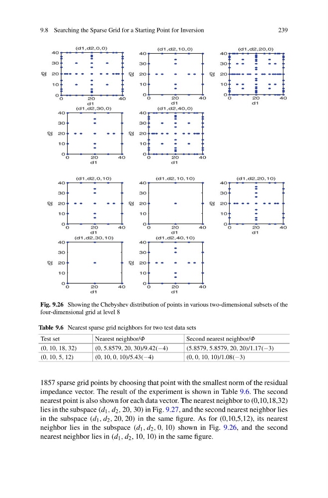
Fig. 9.26 Showing the Chebyshev distribution of points in various two-dimensional subsets of the
four-dimensional grid at level 8
Table 9.6 Nearest sparse grid neighbors for two test data sets
Test set
Nearest neighbor/Φ
Second nearest neighbor/Φ
(0, 10, 18, 32)
(0, 5.8579, 20, 30)/9.42(−4)
(5.8579, 5.8579, 20, 20)/1.17(−3)
(0, 10, 5, 12)
(0, 10, 0, 10)/5.43(−4)
(0, 0, 10, 10)/1.08(−3)
1857 sparse grid points by choosing that point with the smallest norm of the residual
impedance vector. The result of the experiment is shown in Table 9.6. The second
nearest point is also shown for each data vector. The nearest neighbor to (0,10,18,32)
lies in the subspace (d 1 , d 2 , 20, 30) in Fig. 9.27, and the second nearest neighbor lies
in the subspace (d 1 , d 2 , 20, 20) in the same figure. As for (0,10,5,12), its nearest
neighbor lies in the subspace (d 1 , d 2 , 0, 10) shown in Fig. 9.26, and the second
nearest neighbor lies in (d 1 , d 2 , 10, 10) in the same figure.
239
Fig. 9.26 Showing the Chebyshev distribution of points in various two-dimensional subsets of the
four-dimensional grid at level 8
Table 9.6 Nearest sparse grid neighbors for two test data sets
Test set
Nearest neighbor/Φ
Second nearest neighbor/Φ
(0, 10, 18, 32)
(0, 5.8579, 20, 30)/9.42(−4)
(5.8579, 5.8579, 20, 20)/1.17(−3)
(0, 10, 5, 12)
(0, 10, 0, 10)/5.43(−4)
(0, 0, 10, 10)/1.08(−3)
1857 sparse grid points by choosing that point with the smallest norm of the residual
impedance vector. The result of the experiment is shown in Table 9.6. The second
nearest point is also shown for each data vector. The nearest neighbor to (0,10,18,32)
lies in the subspace (d 1 , d 2 , 20, 30) in Fig. 9.27, and the second nearest neighbor lies
in the subspace (d 1 , d 2 , 20, 20) in the same figure. As for (0,10,5,12), its nearest
neighbor lies in the subspace (d 1 , d 2 , 0, 10) shown in Fig. 9.26, and the second
nearest neighbor lies in (d 1 , d 2 , 10, 10) in the same figure.