

9.8 Searching the Sparse Grid for a Starting Point for Inversion
237
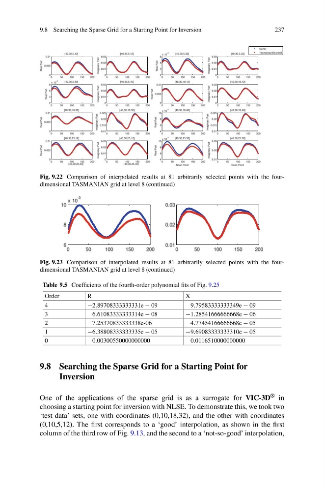
Fig. 9.22 Comparison of interpolated results at 81 arbitrarily selected points with the fourdimensional TASMANIAN grid at level 8 (continued)
Fig. 9.23 Comparison of interpolated results at 81 arbitrarily selected points with the fourdimensional TASMANIAN grid at level 8 (continued)
Table 9.5 Coefficients of the fourth-order polynomial fits of Fig. 9.25
Order
R
X
4
−2.89708333333331e − 09
9.79583333333349e − 09
3
6.61083333333314e − 08
−1.28541666666668e − 06
2
7.25370833333338e-06
4.77454166666668e − 05
1
−6.38808333333335e − 05
−9.69083333333310e − 05
0
0.00300550000000000
0.0116510000000000
9.8 Searching the Sparse Grid for a Starting Point for
Inversion
One of the applications of the sparse grid is as a surrogate for VIC-3D ® in
choosing a starting point for inversion with NLSE. To demonstrate this, we took two
‘test data’ sets, one with coordinates (0,10,18,32), and the other with coordinates
(0,10,5,12). The first corresponds to a ‘good’ interpolation, as shown in the first
column of the third row of Fig. 9.13, and the second to a ‘not-so-good’ interpolation,
237
Fig. 9.22 Comparison of interpolated results at 81 arbitrarily selected points with the fourdimensional TASMANIAN grid at level 8 (continued)
Fig. 9.23 Comparison of interpolated results at 81 arbitrarily selected points with the fourdimensional TASMANIAN grid at level 8 (continued)
Table 9.5 Coefficients of the fourth-order polynomial fits of Fig. 9.25
Order
R
X
4
−2.89708333333331e − 09
9.79583333333349e − 09
3
6.61083333333314e − 08
−1.28541666666668e − 06
2
7.25370833333338e-06
4.77454166666668e − 05
1
−6.38808333333335e − 05
−9.69083333333310e − 05
0
0.00300550000000000
0.0116510000000000
9.8 Searching the Sparse Grid for a Starting Point for
Inversion
One of the applications of the sparse grid is as a surrogate for VIC-3D ® in
choosing a starting point for inversion with NLSE. To demonstrate this, we took two
‘test data’ sets, one with coordinates (0,10,18,32), and the other with coordinates
(0,10,5,12). The first corresponds to a ‘good’ interpolation, as shown in the first
column of the third row of Fig. 9.13, and the second to a ‘not-so-good’ interpolation,