

9.4 The TASMANIAN Sparse Grids Module
227
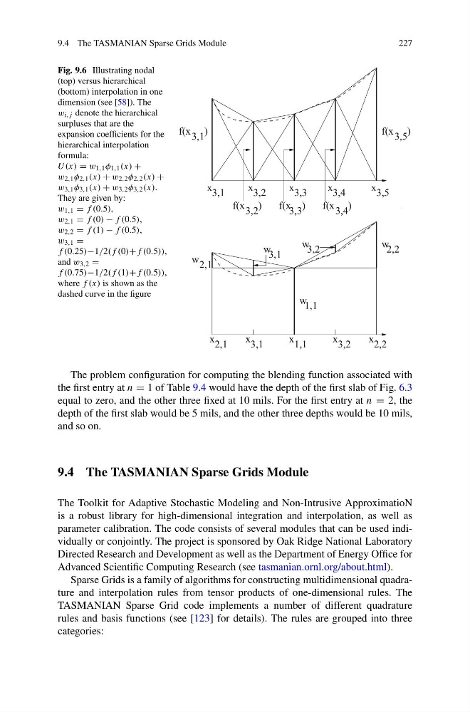
Fig. 9.6 Illustrating nodal
(top) versus hierarchical
(bottom) interpolation in one
dimension (see [58]). The
w i,j denote the hierarchical
surpluses that are the
expansion coefficients for the
hierarchical interpolation
formula:
U(x) = w 1,1 φ 1,1 (x) +
w 2,1 φ 2,1 (x) + w 2,2 φ 2,2 (x) +
w 3,1 φ 3,1 (x) + w 3,2 φ 3,2 (x).
They are given by:
w 1,1 = f (0.5),
w 2,1 = f (0) − f (0.5),
w 2,2 = f (1) − f (0.5),
w 3,1 =
f (0.25)−1/2(f (0)+f (0.5)),
and w 3,2 =
f (0.75)−1/2(f (1)+f (0.5)),
where f (x) is shown as the
dashed curve in the figure
x 3,1
x 3,2
x
x
x
3,3
3,4
3,5
f(x 3,1
)
f(x 3,2 )
f(x 3,3 )
f(x 3,4 )
x
x
x
x
x
2,1
3,1
1,1
3,2
2,2
w
w 3,2
3,1
2,1
w
w 2,2
w
1,1
f(x 3,5
)
The problem configuration for computing the blending function associated with
the first entry at n = 1 of Table 9.4 would have the depth of the first slab of Fig. 6.3
equal to zero, and the other three fixed at 10 mils. For the first entry at n = 2, the
depth of the first slab would be 5 mils, and the other three depths would be 10 mils,
and so on.
9.4 The TASMANIAN Sparse Grids Module
The Toolkit for Adaptive Stochastic Modeling and Non-Intrusive ApproximatioN
is a robust library for high-dimensional integration and interpolation, as well as
parameter calibration. The code consists of several modules that can be used individually or conjointly. The project is sponsored by Oak Ridge National Laboratory
Directed Research and Development as well as the Department of Energy Office for
Advanced Scientific Computing Research (see tasmanian.ornl.org/about.html).
Sparse Grids is a family of algorithms for constructing multidimensional quadrature and interpolation rules from tensor products of one-dimensional rules. The
TASMANIAN Sparse Grid code implements a number of different quadrature
rules and basis functions (see [123] for details). The rules are grouped into three
categories:
227
Fig. 9.6 Illustrating nodal
(top) versus hierarchical
(bottom) interpolation in one
dimension (see [58]). The
w i,j denote the hierarchical
surpluses that are the
expansion coefficients for the
hierarchical interpolation
formula:
U(x) = w 1,1 φ 1,1 (x) +
w 2,1 φ 2,1 (x) + w 2,2 φ 2,2 (x) +
w 3,1 φ 3,1 (x) + w 3,2 φ 3,2 (x).
They are given by:
w 1,1 = f (0.5),
w 2,1 = f (0) − f (0.5),
w 2,2 = f (1) − f (0.5),
w 3,1 =
f (0.25)−1/2(f (0)+f (0.5)),
and w 3,2 =
f (0.75)−1/2(f (1)+f (0.5)),
where f (x) is shown as the
dashed curve in the figure
x 3,1
x 3,2
x
x
x
3,3
3,4
3,5
f(x 3,1
)
f(x 3,2 )
f(x 3,3 )
f(x 3,4 )
x
x
x
x
x
2,1
3,1
1,1
3,2
2,2
w
w 3,2
3,1
2,1
w
w 2,2
w
1,1
f(x 3,5
)
The problem configuration for computing the blending function associated with
the first entry at n = 1 of Table 9.4 would have the depth of the first slab of Fig. 6.3
equal to zero, and the other three fixed at 10 mils. For the first entry at n = 2, the
depth of the first slab would be 5 mils, and the other three depths would be 10 mils,
and so on.
9.4 The TASMANIAN Sparse Grids Module
The Toolkit for Adaptive Stochastic Modeling and Non-Intrusive ApproximatioN
is a robust library for high-dimensional integration and interpolation, as well as
parameter calibration. The code consists of several modules that can be used individually or conjointly. The project is sponsored by Oak Ridge National Laboratory
Directed Research and Development as well as the Department of Energy Office for
Advanced Scientific Computing Research (see tasmanian.ornl.org/about.html).
Sparse Grids is a family of algorithms for constructing multidimensional quadrature and interpolation rules from tensor products of one-dimensional rules. The
TASMANIAN Sparse Grid code implements a number of different quadrature
rules and basis functions (see [123] for details). The rules are grouped into three
categories: