

7.11 Consistency of Calculations
195
consistent with the requirements of the expansion, namely that the random variables
are uncorrelated and have a unit variance.
First, we note that the variance of a random variable that is uniformly distributed
over [0, 1) is 1/12, so that we must multiply the output of RANDOM_NUMBER by
√
12 in order to generate a unit-variance random variable. Secondly, we transform
the range of the output to [−0.5, 0.5) in order to generate a zero-mean random
variable, which will be useful in our later work.
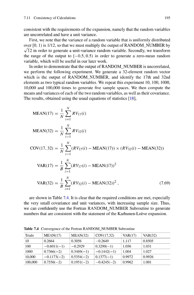
In order to demonstrate that the output of RANDOM_NUMBER is uncorrelated,
we perform the following experiment. We generate a 32-element random vector
which is the output of RANDOM_NUMBER, and identify the 17th and 32nd
elements as two typical random variables. We repeat this experiment 10, 100, 1000,
10,000 and 100,000 times to generate five sample spaces. We then compute the
means and variances of each of the two random variables, as well as their covariance.
The results, obtained using the usual equations of statistics [18],
MEAN(17) =
1
N
N
i=1
RV 17 (i)
MEAN(32) =
1
N
N
i=1
RV 32 (i)
COV(17, 32) =
1
N
N
i=1
(RV 17 (i) − MEAN(17)) × (RV 32 (i) − MEAN(32))
VAR(17) =
1
B
N
i=1
(RV 17 (i) − MEAN(17))
2
VAR(32) =
1
B
N
i=1
(RV 32 (i) − MEAN(32))
2 ,
(7.69)
are shown in Table 7.4. It is clear that the required conditions are met, especially
the very small covariance and unit variances, with increasing sample size. Thus,
we can confidently use the Fortran RANDOM_NUMBER Subroutine to generate
numbers that are consistent with the statement of the Karhunen-Loève expansion.
Table 7.4 Convergence of the Fortran RANDOM_NUMBER Subroutine
Trials
MEAN(17)
MEAN(32)
COV(17,32)
VAR(17)
VAR(32)
10
0.2664
0.3056
−0.2649
1.117
0.8505
100
−0.6011(−1)
−0.2929
0.3290(−1)
1.056
1.031
1000
0.7366(−2)
0.3469(−1)
−0.1442(−1)
1.004
1.027
10,000
−0.1173(−2)
0.5354(−2)
0.1377(−1)
0.9972
0.9926
100,000
0.7556(−2)
0.1951(−2)
−0.4245(−2)
0.9962
1.001
195
consistent with the requirements of the expansion, namely that the random variables
are uncorrelated and have a unit variance.
First, we note that the variance of a random variable that is uniformly distributed
over [0, 1) is 1/12, so that we must multiply the output of RANDOM_NUMBER by
√
12 in order to generate a unit-variance random variable. Secondly, we transform
the range of the output to [−0.5, 0.5) in order to generate a zero-mean random
variable, which will be useful in our later work.
In order to demonstrate that the output of RANDOM_NUMBER is uncorrelated,
we perform the following experiment. We generate a 32-element random vector
which is the output of RANDOM_NUMBER, and identify the 17th and 32nd
elements as two typical random variables. We repeat this experiment 10, 100, 1000,
10,000 and 100,000 times to generate five sample spaces. We then compute the
means and variances of each of the two random variables, as well as their covariance.
The results, obtained using the usual equations of statistics [18],
MEAN(17) =
1
N
N
i=1
RV 17 (i)
MEAN(32) =
1
N
N
i=1
RV 32 (i)
COV(17, 32) =
1
N
N
i=1
(RV 17 (i) − MEAN(17)) × (RV 32 (i) − MEAN(32))
VAR(17) =
1
B
N
i=1
(RV 17 (i) − MEAN(17))
2
VAR(32) =
1
B
N
i=1
(RV 32 (i) − MEAN(32))
2 ,
(7.69)
are shown in Table 7.4. It is clear that the required conditions are met, especially
the very small covariance and unit variances, with increasing sample size. Thus,
we can confidently use the Fortran RANDOM_NUMBER Subroutine to generate
numbers that are consistent with the statement of the Karhunen-Loève expansion.
Table 7.4 Convergence of the Fortran RANDOM_NUMBER Subroutine
Trials
MEAN(17)
MEAN(32)
COV(17,32)
VAR(17)
VAR(32)
10
0.2664
0.3056
−0.2649
1.117
0.8505
100
−0.6011(−1)
−0.2929
0.3290(−1)
1.056
1.031
1000
0.7366(−2)
0.3469(−1)
−0.1442(−1)
1.004
1.027
10,000
−0.1173(−2)
0.5354(−2)
0.1377(−1)
0.9972
0.9926
100,000
0.7556(−2)
0.1951(−2)
−0.4245(−2)
0.9962
1.001