

174
7 Integration of Functionals, PCM and Stochastic IntegralEquations
0
100000
200000
300000
400000
500000
600000
0
5
10
15
20
25
30
35
Ten conductivity profiles for L/delta=1
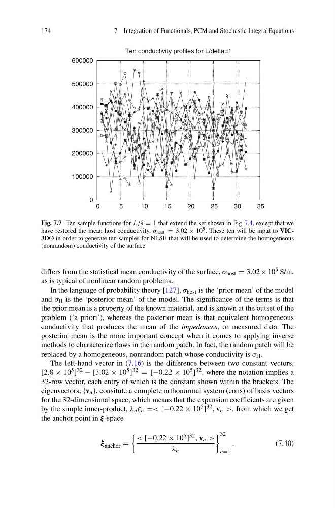
Fig. 7.7 Ten sample functions for L/δ = 1 that extend the set shown in Fig. 7.4, except that we
have restored the mean host conductivity, σ host = 3.02 × 10 5 . These ten will be input to VIC3D® in order to generate ten samples for NLSE that will be used to determine the homogeneous
(nonrandom) conductivity of the surface
differs from the statistical mean conductivity of the surface, σ host = 3.02 × 10 5 S/m,
as is typical of nonlinear random problems.
In the language of probability theory [127], σ host is the ‘prior mean’ of the model
and σ H is the ‘posterior mean’ of the model. The significance of the terms is that
the prior mean is a property of the known material, and is known at the outset of the
problem (‘a priori’), whereas the posterior mean is that equivalent homogeneous
conductivity that produces the mean of the impedances, or measured data. The
posterior mean is the more important concept when it comes to applying inverse
methods to characterize flaws in the random patch. In fact, the random patch will be
replaced by a homogeneous, nonrandom patch whose conductivity is σ H .
The left-hand vector in (7.16) is the difference between two constant vectors,
[2.8 × 10 5 ] 32 − [3.02 × 10 5 ] 32 = [−0.22 × 10 5 ] 32 , where the notation implies a
32-row vector, each entry of which is the constant shown within the brackets. The
eigenvectors, {v n }, consitute a complete orthonormal system (cons) of basis vectors
for the 32-dimensional space, which means that the expansion coefficients are given
by the simple inner-product, λ n ξ n =< [−0.22 × 10 5 ] 32 , v n >, from which we get
the anchor point in ξ -space
ξ anchor =
< [−0.22 × 10 5 ] 32 , v n >
λ n
32
n=1
.
(7.40)
7 Integration of Functionals, PCM and Stochastic IntegralEquations
0
100000
200000
300000
400000
500000
600000
0
5
10
15
20
25
30
35
Ten conductivity profiles for L/delta=1
Fig. 7.7 Ten sample functions for L/δ = 1 that extend the set shown in Fig. 7.4, except that we
have restored the mean host conductivity, σ host = 3.02 × 10 5 . These ten will be input to VIC3D® in order to generate ten samples for NLSE that will be used to determine the homogeneous
(nonrandom) conductivity of the surface
differs from the statistical mean conductivity of the surface, σ host = 3.02 × 10 5 S/m,
as is typical of nonlinear random problems.
In the language of probability theory [127], σ host is the ‘prior mean’ of the model
and σ H is the ‘posterior mean’ of the model. The significance of the terms is that
the prior mean is a property of the known material, and is known at the outset of the
problem (‘a priori’), whereas the posterior mean is that equivalent homogeneous
conductivity that produces the mean of the impedances, or measured data. The
posterior mean is the more important concept when it comes to applying inverse
methods to characterize flaws in the random patch. In fact, the random patch will be
replaced by a homogeneous, nonrandom patch whose conductivity is σ H .
The left-hand vector in (7.16) is the difference between two constant vectors,
[2.8 × 10 5 ] 32 − [3.02 × 10 5 ] 32 = [−0.22 × 10 5 ] 32 , where the notation implies a
32-row vector, each entry of which is the constant shown within the brackets. The
eigenvectors, {v n }, consitute a complete orthonormal system (cons) of basis vectors
for the 32-dimensional space, which means that the expansion coefficients are given
by the simple inner-product, λ n ξ n =< [−0.22 × 10 5 ] 32 , v n >, from which we get
the anchor point in ξ -space
ξ anchor =
< [−0.22 × 10 5 ] 32 , v n >
λ n
32
n=1
.
(7.40)