

7.6 HDMR and ANOVA
171
where, if the ‘density measure’ dμ(x) = dx, results in the usual expression for an
average
Pf (x) =
f (x)dx .
(7.30)
If dμ(x) = δ(x − a)dx, where δ(x − a) is the one-dimensional Dirac delta function
centered at x = a, then the average is simply given by the evaluation of f (x) at
x = a:
Pf (x) =
f (x)δ(x − a)dx = f (a) .
(7.31)
From here on we will work in the M−dimensional Dirac measure, δ(x 1 − a 1 )δ(x 2 −
a 2 ) · · · δ(x M − a M ) where a is the M−dimensional ‘anchor point’ of the expansion.
Decompose the M−dimensional identity operator into the tensor product of M
one-dimensional operators:
I
(M)
= ⊗
M
j =1
P j + (I j − P j )
=
i
P i +
i
(I i − P i )
i =j
P j
+
i
k =i,j
P k + · · · +
i
(I i − P i ) ,
(7.32)
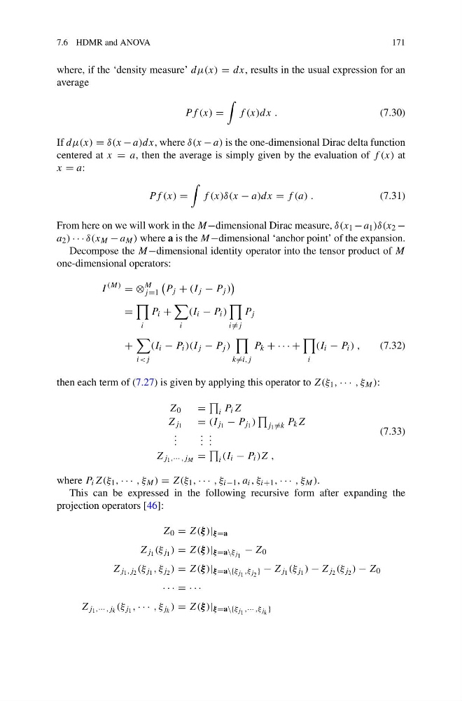
then each term of (7.27) is given by applying this operator to Z(ξ 1 , · · · , ξ M ):
Z 0
=
i P i Z
Z j 1
= (I j 1 − P j 1 )
j 1 =k P k Z
. . .
. . .
. . .
Z j 1 ,··· ,j M =
i (I i − P i )Z ,
(7.33)
where P i Z(ξ 1 , · · · , ξ M ) = Z(ξ 1 , · · · , ξ i−1 , a i , ξ i+1 , · · · , ξ M ).
This can be expressed in the following recursive form after expanding the
projection operators [46]:
Z 0 = Z(ξ )| ξ =a
Z j 1 (ξ j 1 ) = Z(ξ )| ξ =a\ξ j 1 − Z 0
Z j 1 ,j 2 (ξ j 1 , ξ j 2 ) = Z(ξ )| ξ =a\{ξ j 1 ,ξ j 2 } − Z j 1 (ξ j 1 ) − Z j 2 (ξ j 2 ) − Z 0
· · · = · · ·
Z j 1 ,··· ,j k (ξ j 1 , · · · , ξ j k ) = Z(ξ )| ξ =a\{ξ j 1 ,··· ,ξ j k }
171
where, if the ‘density measure’ dμ(x) = dx, results in the usual expression for an
average
Pf (x) =
f (x)dx .
(7.30)
If dμ(x) = δ(x − a)dx, where δ(x − a) is the one-dimensional Dirac delta function
centered at x = a, then the average is simply given by the evaluation of f (x) at
x = a:
Pf (x) =
f (x)δ(x − a)dx = f (a) .
(7.31)
From here on we will work in the M−dimensional Dirac measure, δ(x 1 − a 1 )δ(x 2 −
a 2 ) · · · δ(x M − a M ) where a is the M−dimensional ‘anchor point’ of the expansion.
Decompose the M−dimensional identity operator into the tensor product of M
one-dimensional operators:
I
(M)
= ⊗
M
j =1
P j + (I j − P j )
=
i
P i +
i
(I i − P i )
i =j
P j
+
i
k =i,j
P k + · · · +
i
(I i − P i ) ,
(7.32)
then each term of (7.27) is given by applying this operator to Z(ξ 1 , · · · , ξ M ):
Z 0
=
i P i Z
Z j 1
= (I j 1 − P j 1 )
j 1 =k P k Z
. . .
. . .
. . .
Z j 1 ,··· ,j M =
i (I i − P i )Z ,
(7.33)
where P i Z(ξ 1 , · · · , ξ M ) = Z(ξ 1 , · · · , ξ i−1 , a i , ξ i+1 , · · · , ξ M ).
This can be expressed in the following recursive form after expanding the
projection operators [46]:
Z 0 = Z(ξ )| ξ =a
Z j 1 (ξ j 1 ) = Z(ξ )| ξ =a\ξ j 1 − Z 0
Z j 1 ,j 2 (ξ j 1 , ξ j 2 ) = Z(ξ )| ξ =a\{ξ j 1 ,ξ j 2 } − Z j 1 (ξ j 1 ) − Z j 2 (ξ j 2 ) − Z 0
· · · = · · ·
Z j 1 ,··· ,j k (ξ j 1 , · · · , ξ j k ) = Z(ξ )| ξ =a\{ξ j 1 ,··· ,ξ j k }