

138
5 An Electromagnetic Model for Anisotropic Media: Green’s Dyad for Plane-. . .
-0.15
-0.1
-0.05
0
0.05
0.1
0
50
100
150
200
250
300
350
400
R
Rotation Angle (Deg)
Interpolation Blending Functions
A
B
C
D
-0.4
-0.3
-0.2
-0.1
0
0.1
0.2
0.3
0.4
0.5
0
50
100
150
200
250
300
350
400
X
Rotation Angle (Deg)
Interpolation Blending Functions
A
B
C
D
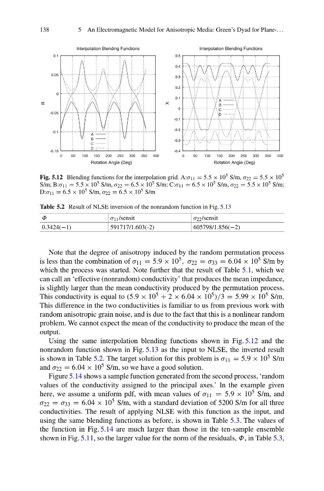
Fig. 5.12 Blending functions for the interpolation grid. A:σ 11 = 5.5 × 10 5 S/m, σ 22 = 5.5 × 10 5
S/m; B:σ 11 = 5.5 × 10 5 S/m, σ 22 = 6.5 × 10 5 S/m; C:σ 11 = 6.5 × 10 5 S/m, σ 22 = 5.5 × 10 5 S/m;
D:σ 11 = 6.5 × 10 5 S/m, σ 22 = 6.5 × 10 5 S/m
Table 5.2 Result of NLSE inversion of the nonrandom function in Fig. 5.13
Φ
σ 11 /sensit
σ 22 /sensit
0.3424(−1)
591717/1.603(-2)
605798/1.856(−2)
Note that the degree of anisotropy induced by the random permutation process
is less than the combination of σ 11 = 5.9 × 10 5 , σ 22 = σ 33 = 6.04 × 10 5 S/m by
which the process was started. Note further that the result of Table 5.1, which we
can call an ‘effective (nonrandom) conductivity’ that produces the mean impedance,
is slightly larger than the mean conductivity produced by the permutation process.
This conductivity is equal to (5.9 × 10 5 + 2 × 6.04 × 10 5 )/3 = 5.99 × 10 5 S/m.
This difference in the two conductivities is familiar to us from previous work with
random anisotropic grain noise, and is due to the fact that this is a nonlinear random
problem. We cannot expect the mean of the conductivity to produce the mean of the
output.
Using the same interpolation blending functions shown in Fig. 5.12 and the
nonrandom function shown in Fig. 5.13 as the input to NLSE, the inverted result
is shown in Table 5.2. The target solution for this problem is σ 11 = 5.9 × 10 5 S/m
and σ 22 = 6.04 × 10 5 S/m, so we have a good solution.
Figure 5.14 shows a sample function generated from the second process, ‘random
values of the conductivity assigned to the principal axes.’ In the example given
here, we assume a uniform pdf, with mean values of σ 11 = 5.9 × 10 5 S/m, and
σ 22 = σ 33 = 6.04 × 10 5 S/m, with a standard deviation of 5200 S/m for all three
conductivities. The result of applying NLSE with this function as the input, and
using the same blending functions as before, is shown in Table 5.3. The values of
the function in Fig. 5.14 are much larger than those in the ten-sample ensemble
shown in Fig. 5.11, so the larger value for the norm of the residuals, Φ, in Table 5.3,
5 An Electromagnetic Model for Anisotropic Media: Green’s Dyad for Plane-. . .
-0.15
-0.1
-0.05
0
0.05
0.1
0
50
100
150
200
250
300
350
400
R
Rotation Angle (Deg)
Interpolation Blending Functions
A
B
C
D
-0.4
-0.3
-0.2
-0.1
0
0.1
0.2
0.3
0.4
0.5
0
50
100
150
200
250
300
350
400
X
Rotation Angle (Deg)
Interpolation Blending Functions
A
B
C
D
Fig. 5.12 Blending functions for the interpolation grid. A:σ 11 = 5.5 × 10 5 S/m, σ 22 = 5.5 × 10 5
S/m; B:σ 11 = 5.5 × 10 5 S/m, σ 22 = 6.5 × 10 5 S/m; C:σ 11 = 6.5 × 10 5 S/m, σ 22 = 5.5 × 10 5 S/m;
D:σ 11 = 6.5 × 10 5 S/m, σ 22 = 6.5 × 10 5 S/m
Table 5.2 Result of NLSE inversion of the nonrandom function in Fig. 5.13
Φ
σ 11 /sensit
σ 22 /sensit
0.3424(−1)
591717/1.603(-2)
605798/1.856(−2)
Note that the degree of anisotropy induced by the random permutation process
is less than the combination of σ 11 = 5.9 × 10 5 , σ 22 = σ 33 = 6.04 × 10 5 S/m by
which the process was started. Note further that the result of Table 5.1, which we
can call an ‘effective (nonrandom) conductivity’ that produces the mean impedance,
is slightly larger than the mean conductivity produced by the permutation process.
This conductivity is equal to (5.9 × 10 5 + 2 × 6.04 × 10 5 )/3 = 5.99 × 10 5 S/m.
This difference in the two conductivities is familiar to us from previous work with
random anisotropic grain noise, and is due to the fact that this is a nonlinear random
problem. We cannot expect the mean of the conductivity to produce the mean of the
output.
Using the same interpolation blending functions shown in Fig. 5.12 and the
nonrandom function shown in Fig. 5.13 as the input to NLSE, the inverted result
is shown in Table 5.2. The target solution for this problem is σ 11 = 5.9 × 10 5 S/m
and σ 22 = 6.04 × 10 5 S/m, so we have a good solution.
Figure 5.14 shows a sample function generated from the second process, ‘random
values of the conductivity assigned to the principal axes.’ In the example given
here, we assume a uniform pdf, with mean values of σ 11 = 5.9 × 10 5 S/m, and
σ 22 = σ 33 = 6.04 × 10 5 S/m, with a standard deviation of 5200 S/m for all three
conductivities. The result of applying NLSE with this function as the input, and
using the same blending functions as before, is shown in Table 5.3. The values of
the function in Fig. 5.14 are much larger than those in the ten-sample ensemble
shown in Fig. 5.11, so the larger value for the norm of the residuals, Φ, in Table 5.3,