

116
4 Application of the Set-Theoretic Algorithm to CFRP’s
4.7 Progress in Modeling Microstructure Quantification
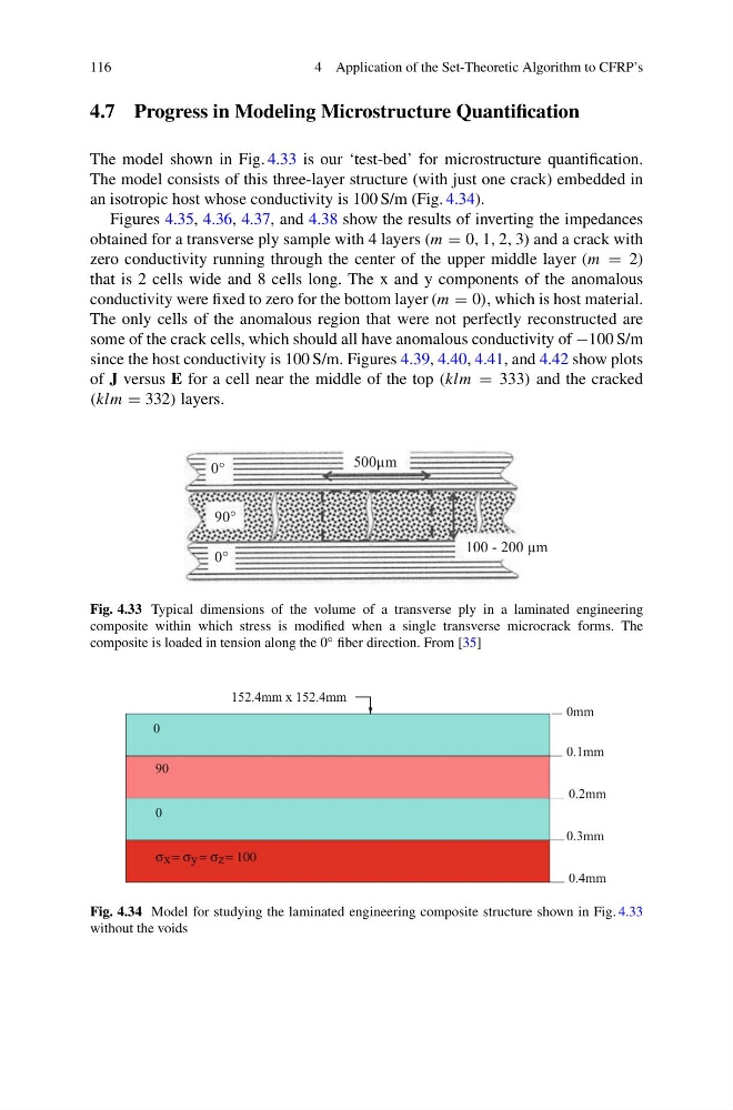
The model shown in Fig. 4.33 is our ‘test-bed’ for microstructure quantification.
The model consists of this three-layer structure (with just one crack) embedded in
an isotropic host whose conductivity is 100 S/m (Fig. 4.34).
Figures 4.35, 4.36, 4.37, and 4.38 show the results of inverting the impedances
obtained for a transverse ply sample with 4 layers (m = 0, 1, 2, 3) and a crack with
zero conductivity running through the center of the upper middle layer (m = 2)
that is 2 cells wide and 8 cells long. The x and y components of the anomalous
conductivity were fixed to zero for the bottom layer (m = 0), which is host material.
The only cells of the anomalous region that were not perfectly reconstructed are
some of the crack cells, which should all have anomalous conductivity of −100 S/m
since the host conductivity is 100 S/m. Figures 4.39, 4.40, 4.41, and 4.42 show plots
of J versus E for a cell near the middle of the top (klm = 333) and the cracked
(klm = 332) layers.
500µm
0°
0°
90°
100 - 200 µm
Fig. 4.33 Typical dimensions of the volume of a transverse ply in a laminated engineering
composite within which stress is modified when a single transverse microcrack forms. The
composite is loaded in tension along the 0 ◦ fiber direction. From [35]
0
90
0
0mm
0.1mm
0.2mm
0.3mm
0.4mm
152.4mm x 152.4mm
x
y
σ = σ = σ = 100
z
Fig. 4.34 Model for studying the laminated engineering composite structure shown in Fig. 4.33
without the voids
4 Application of the Set-Theoretic Algorithm to CFRP’s
4.7 Progress in Modeling Microstructure Quantification
The model shown in Fig. 4.33 is our ‘test-bed’ for microstructure quantification.
The model consists of this three-layer structure (with just one crack) embedded in
an isotropic host whose conductivity is 100 S/m (Fig. 4.34).
Figures 4.35, 4.36, 4.37, and 4.38 show the results of inverting the impedances
obtained for a transverse ply sample with 4 layers (m = 0, 1, 2, 3) and a crack with
zero conductivity running through the center of the upper middle layer (m = 2)
that is 2 cells wide and 8 cells long. The x and y components of the anomalous
conductivity were fixed to zero for the bottom layer (m = 0), which is host material.
The only cells of the anomalous region that were not perfectly reconstructed are
some of the crack cells, which should all have anomalous conductivity of −100 S/m
since the host conductivity is 100 S/m. Figures 4.39, 4.40, 4.41, and 4.42 show plots
of J versus E for a cell near the middle of the top (klm = 333) and the cracked
(klm = 332) layers.
500µm
0°
0°
90°
100 - 200 µm
Fig. 4.33 Typical dimensions of the volume of a transverse ply in a laminated engineering
composite within which stress is modified when a single transverse microcrack forms. The
composite is loaded in tension along the 0 ◦ fiber direction. From [35]
0
90
0
0mm
0.1mm
0.2mm
0.3mm
0.4mm
152.4mm x 152.4mm
x
y
σ = σ = σ = 100
z
Fig. 4.34 Model for studying the laminated engineering composite structure shown in Fig. 4.33
without the voids