

4.3 An Anisotropic Inverse Problem for Measuring FAWT
93
4.3.2 Second Set-Theoretic Result
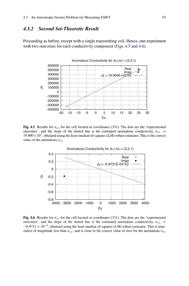
Proceeding as before, except with a single transmitting coil. Hence, one experiment
with two outcomes for each conductivity component (Figs. 4.5 and 4.6).
-400000
-300000
-200000
-100000
0
100000
200000
300000
400000
500000
600000
-20 -15 -10 -5
0
5
10 15 20 25 30
Jx
Ex
Anomalous Conductivity for (k,l,m) = (3,3,1)
Real
Imag
Jx = 19.900E+03*Ex
Fig. 4.5 Results for σ xx for the cell located at coordinates (331). The dots are the ‘experimental
outcomes’, and the slope of the dotted line is the estimated anomalous conductivity, σ xx =
19.900×10 3 , obtained using the least-median-of-squares (LM) robust estimator. This is the correct
value of the anomalous σ xx
-0.8
-0.6
-0.4
-0.2
0
0.2
0.4
-4000 -3000 -2000 -1000
0
1000 2000 3000 4000
Jy
Ey
Anomalous Conductivity for (k,l,m) = (3,3,1)
Real
Imag
Jy = -0.9731E-04*Ey
Fig. 4.6 Results for σ yy for the cell located at coordinates (331). The dots are the ‘experimental
outcomes’, and the slope of the dotted line is the estimated anomalous conductivity, σ yy =
−0.9731 × 10 −4 , obtained using the least-median-of-squares (LM) robust estimator. This is nineorders of magnitude less than σ xx , and is close to the correct value of zero for the anomalous σ yy
93
4.3.2 Second Set-Theoretic Result
Proceeding as before, except with a single transmitting coil. Hence, one experiment
with two outcomes for each conductivity component (Figs. 4.5 and 4.6).
-400000
-300000
-200000
-100000
0
100000
200000
300000
400000
500000
600000
-20 -15 -10 -5
0
5
10 15 20 25 30
Jx
Ex
Anomalous Conductivity for (k,l,m) = (3,3,1)
Real
Imag
Jx = 19.900E+03*Ex
Fig. 4.5 Results for σ xx for the cell located at coordinates (331). The dots are the ‘experimental
outcomes’, and the slope of the dotted line is the estimated anomalous conductivity, σ xx =
19.900×10 3 , obtained using the least-median-of-squares (LM) robust estimator. This is the correct
value of the anomalous σ xx
-0.8
-0.6
-0.4
-0.2
0
0.2
0.4
-4000 -3000 -2000 -1000
0
1000 2000 3000 4000
Jy
Ey
Anomalous Conductivity for (k,l,m) = (3,3,1)
Real
Imag
Jy = -0.9731E-04*Ey
Fig. 4.6 Results for σ yy for the cell located at coordinates (331). The dots are the ‘experimental
outcomes’, and the slope of the dotted line is the estimated anomalous conductivity, σ yy =
−0.9731 × 10 −4 , obtained using the least-median-of-squares (LM) robust estimator. This is nineorders of magnitude less than σ xx , and is close to the correct value of zero for the anomalous σ yy