

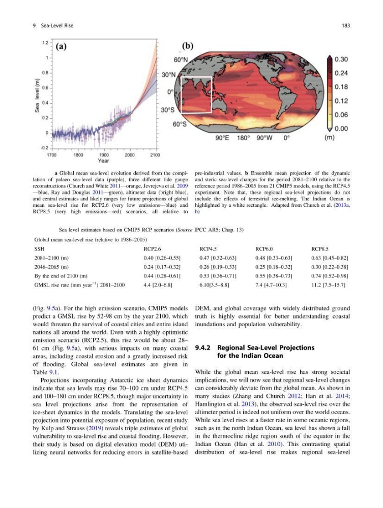
(Fig. 9.5a). For the high emission scenario, CMIP5 models
predict a GMSL rise by 52-98 cm by the year 2100, which
would threaten the survival of coastal cities and entire island
nations all around the world. Even with a highly optimistic
emission scenario (RCP2.5), this rise would be about 28–
61 cm (Fig. 9.5a), with serious impacts on many coastal
areas, including coastal erosion and a greatly increased risk
of flooding. Global sea-level estimates are given in
Table 9.1.
Projections incorporating Antarctic ice sheet dynamics
indicate that sea levels may rise 70–100 cm under RCP4.5
and 100–180 cm under RCP8.5, though major uncertainty in
sea level projections arise from the representation of
ice-sheet dynamics in the models. Translating the sea-level
projection into potential exposure of population, recent study
by Kulp and Strauss (2019) reveals triple estimates of global
vulnerability to sea-level rise and coastal flooding. However,
their study is based on digital elevation model (DEM) utilizing neural networks for reducing errors in satellite-based
DEM, and global coverage with widely distributed ground
truth is highly essential for better understanding coastal
inundations and population vulnerability.
9.4.2 Regional Sea-Level Projections
for the Indian Ocean
While the global mean sea-level rise has strong societal
implications, we will now see that regional sea-level changes
can considerably deviate from the global mean. As shown in
many studies (Zhang and Church 2012; Han et al. 2014;
Hamlington et al. 2013), the observed sea-level rise over the
altimeter period is indeed not uniform over the world oceans.
While sea level rises at a faster rate in some oceanic regions,
such as in the north Indian Ocean, sea level has shown a fall
in the thermocline ridge region south of the equator in the
Indian Ocean (Han et al. 2010). This contrasting spatial
distribution of sea-level rise makes regional sea-level
Fig. 9.5 a Global mean sea-level evolution derived from the compilation of palaeo sea-level data (purple), three different tide gauge
reconstructions (Church and White 2011—orange, Jevrejeva et al. 2009
—blue, Ray and Douglas 2011—green), altimeter data (bright blue),
and central estimates and likely ranges for future projections of global
mean sea-level rise for RCP2.6 (very low emissions—blue) and
RCP8.5 (very high emissions—red) scenarios, all relative to
pre-industrial values. b Ensemble mean projection of the dynamic
and steric sea-level changes for the period 2081–2100 relative to the
reference period 1986–2005 from 21 CMIP5 models, using the RCP4.5
experiment. Note that, these regional sea-level projections do not
include the effects of terrestrial ice-melting. The Indian Ocean is
highlighted by a white rectangle. Adapted from Church et al. (2013a,
b)
Table 9.1 Sea level estimates based on CMIP5 RCP scenarios (Source IPCC AR5; Chap. 13)
Global mean sea-level rise (relative to 1986–2005)
SSH
RCP2.6
RCP4.5
RCP6.0
RCP8.5
2081–2100 (m)
0.40 [0.26–0.55]
0.47 [0.32–0.63]
0.48 [0.33–0.63]
0.63 [0.45–0.82]
2046–2065 (m)
0.24 [0.17–0.32]
0.26 [0.19–0.33]
0.25 [0.18–0.32]
0.30 [0.22–0.38]
By the end of 2100 (m)
0.44 [0.28–0.61]
0.53 [0.36–0.71]
0.55 [0.38–0.73]
0.74 [0.52–0.98]
GMSL rise rate (mm year
−1
) 2081–2100
4.4 [2.0–6.8]
6.10[3.5–8.8]
7.4 [4.7–10.3]
11.2 [7.5–15.7]
9 Sea-Level Rise
183
predict a GMSL rise by 52-98 cm by the year 2100, which
would threaten the survival of coastal cities and entire island
nations all around the world. Even with a highly optimistic
emission scenario (RCP2.5), this rise would be about 28–
61 cm (Fig. 9.5a), with serious impacts on many coastal
areas, including coastal erosion and a greatly increased risk
of flooding. Global sea-level estimates are given in
Table 9.1.
Projections incorporating Antarctic ice sheet dynamics
indicate that sea levels may rise 70–100 cm under RCP4.5
and 100–180 cm under RCP8.5, though major uncertainty in
sea level projections arise from the representation of
ice-sheet dynamics in the models. Translating the sea-level
projection into potential exposure of population, recent study
by Kulp and Strauss (2019) reveals triple estimates of global
vulnerability to sea-level rise and coastal flooding. However,
their study is based on digital elevation model (DEM) utilizing neural networks for reducing errors in satellite-based
DEM, and global coverage with widely distributed ground
truth is highly essential for better understanding coastal
inundations and population vulnerability.
9.4.2 Regional Sea-Level Projections
for the Indian Ocean
While the global mean sea-level rise has strong societal
implications, we will now see that regional sea-level changes
can considerably deviate from the global mean. As shown in
many studies (Zhang and Church 2012; Han et al. 2014;
Hamlington et al. 2013), the observed sea-level rise over the
altimeter period is indeed not uniform over the world oceans.
While sea level rises at a faster rate in some oceanic regions,
such as in the north Indian Ocean, sea level has shown a fall
in the thermocline ridge region south of the equator in the
Indian Ocean (Han et al. 2010). This contrasting spatial
distribution of sea-level rise makes regional sea-level
Fig. 9.5 a Global mean sea-level evolution derived from the compilation of palaeo sea-level data (purple), three different tide gauge
reconstructions (Church and White 2011—orange, Jevrejeva et al. 2009
—blue, Ray and Douglas 2011—green), altimeter data (bright blue),
and central estimates and likely ranges for future projections of global
mean sea-level rise for RCP2.6 (very low emissions—blue) and
RCP8.5 (very high emissions—red) scenarios, all relative to
pre-industrial values. b Ensemble mean projection of the dynamic
and steric sea-level changes for the period 2081–2100 relative to the
reference period 1986–2005 from 21 CMIP5 models, using the RCP4.5
experiment. Note that, these regional sea-level projections do not
include the effects of terrestrial ice-melting. The Indian Ocean is
highlighted by a white rectangle. Adapted from Church et al. (2013a,
b)
Table 9.1 Sea level estimates based on CMIP5 RCP scenarios (Source IPCC AR5; Chap. 13)
Global mean sea-level rise (relative to 1986–2005)
SSH
RCP2.6
RCP4.5
RCP6.0
RCP8.5
2081–2100 (m)
0.40 [0.26–0.55]
0.47 [0.32–0.63]
0.48 [0.33–0.63]
0.63 [0.45–0.82]
2046–2065 (m)
0.24 [0.17–0.32]
0.26 [0.19–0.33]
0.25 [0.18–0.32]
0.30 [0.22–0.38]
By the end of 2100 (m)
0.44 [0.28–0.61]
0.53 [0.36–0.71]
0.55 [0.38–0.73]
0.74 [0.52–0.98]
GMSL rise rate (mm year
−1
) 2081–2100
4.4 [2.0–6.8]
6.10[3.5–8.8]
7.4 [4.7–10.3]
11.2 [7.5–15.7]
9 Sea-Level Rise
183