

7.5 Student’s t-Distribution
81
from the root of numbers drawn from a χ
2 -distribution. Note that originally we start
from n samples or independent measurements and one degree of freedom was used
to determine the average ¯
X n . Therefore the estimate of the variance S n only contains
information of ν = n − 1 degrees of freedom. The χ
2
−distribution that we need to
consider is therefore one for ν = n − 1 degrees of freedom.
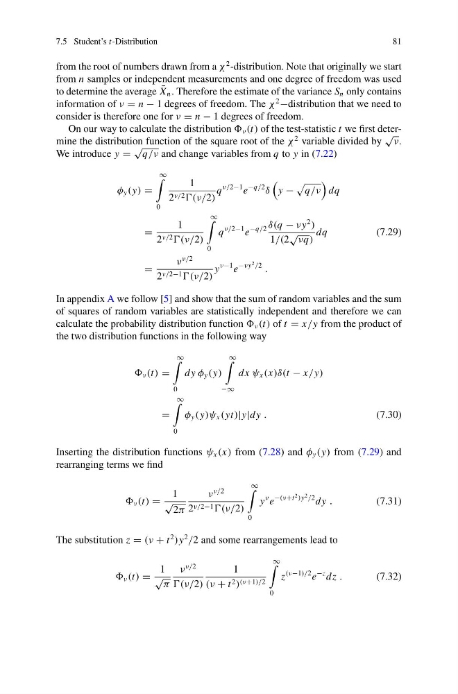
On our way to calculate the distribution ν (t) of the test-statistic t we first determine the distribution function of the square root of the χ
2 variable divided by
√ ν.
We introduce y =
√
q/ν and change variables from q to y in (7.22)
φ y (y) =
∞
0
1
2 ν/2 (ν/2)
q
ν/2−1 e
−q/2
δ
y −
q/ν
dq
=
1
2 ν/2 (ν/2)
∞
0
q
ν/2−1 e
−q/2 δ(q − νy
2
)
1/(2
√ νq)
dq
(7.29)
=
ν
ν/2
2 ν/2−1 (ν/2)
y
ν−1 e
−νy
2 /2
.
In appendix A we follow [5] and show that the sum of random variables and the sum
of squares of random variables are statistically independent and therefore we can
calculate the probability distribution function ν (t) of t = x/y from the product of
the two distribution functions in the following way
ν (t) =
∞
0
dy φ y (y)
∞
−∞
dx ψ x (x)δ(t − x/y)
=
∞
0
φ y (y)ψ x (yt)|y|dy .
(7.30)
Inserting the distribution functions ψ x (x) from (7.28) and φ y (y) from (7.29) and
rearranging terms we find
ν (t) =
1
√
2π
ν
ν/2
2 ν/2−1 (ν/2)
∞
0
y
ν e
−(ν+t
2 )y
2 /2 dy .
(7.31)
The substitution z = (ν + t
2
)y
2
/2 and some rearrangements lead to
ν (t) =
1
√ π
ν
ν/2
(ν/2)
1
(ν + t 2 ) (ν+1)/2
∞
0
z
(ν−1)/2 e
−z dz .
(7.32)
81
from the root of numbers drawn from a χ
2 -distribution. Note that originally we start
from n samples or independent measurements and one degree of freedom was used
to determine the average ¯
X n . Therefore the estimate of the variance S n only contains
information of ν = n − 1 degrees of freedom. The χ
2
−distribution that we need to
consider is therefore one for ν = n − 1 degrees of freedom.
On our way to calculate the distribution ν (t) of the test-statistic t we first determine the distribution function of the square root of the χ
2 variable divided by
√ ν.
We introduce y =
√
q/ν and change variables from q to y in (7.22)
φ y (y) =
∞
0
1
2 ν/2 (ν/2)
q
ν/2−1 e
−q/2
δ
y −
q/ν
dq
=
1
2 ν/2 (ν/2)
∞
0
q
ν/2−1 e
−q/2 δ(q − νy
2
)
1/(2
√ νq)
dq
(7.29)
=
ν
ν/2
2 ν/2−1 (ν/2)
y
ν−1 e
−νy
2 /2
.
In appendix A we follow [5] and show that the sum of random variables and the sum
of squares of random variables are statistically independent and therefore we can
calculate the probability distribution function ν (t) of t = x/y from the product of
the two distribution functions in the following way
ν (t) =
∞
0
dy φ y (y)
∞
−∞
dx ψ x (x)δ(t − x/y)
=
∞
0
φ y (y)ψ x (yt)|y|dy .
(7.30)
Inserting the distribution functions ψ x (x) from (7.28) and φ y (y) from (7.29) and
rearranging terms we find
ν (t) =
1
√
2π
ν
ν/2
2 ν/2−1 (ν/2)
∞
0
y
ν e
−(ν+t
2 )y
2 /2 dy .
(7.31)
The substitution z = (ν + t
2
)y
2
/2 and some rearrangements lead to
ν (t) =
1
√ π
ν
ν/2
(ν/2)
1
(ν + t 2 ) (ν+1)/2
∞
0
z
(ν−1)/2 e
−z dz .
(7.32)