

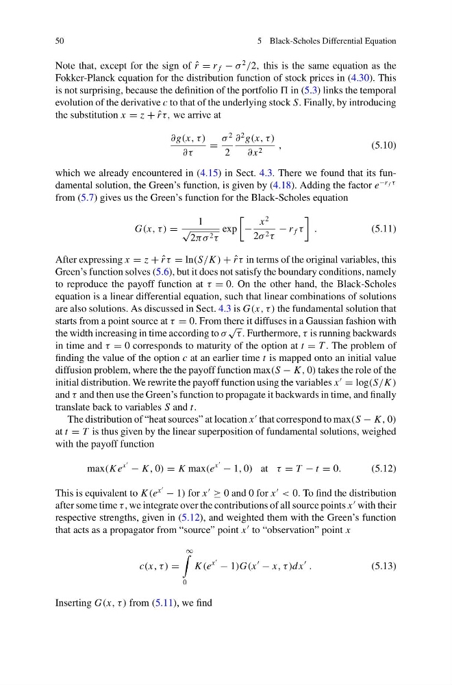
50
5 Black-Scholes Differential Equation
Note that, except for the sign of ˆ
r = r f − σ
2
/2, this is the same equation as the
Fokker-Planck equation for the distribution function of stock prices in (4.30). This
is not surprising, because the definition of the portfolio in (5.3) links the temporal
evolution of the derivative c to that of the underlying stock S. Finally, by introducing
the substitution x = z + ˆ
r τ, we arrive at
∂g(x, τ )
∂τ
=
σ
2
2
∂
2 g(x, τ )
∂ x 2
,
(5.10)
which we already encountered in (4.15) in Sect. 4.3. There we found that its fundamental solution, the Green’s function, is given by (4.18). Adding the factor e
−r f τ
from (5.7) gives us the Green’s function for the Black-Scholes equation
G(x, τ ) =
1
√
2πσ 2 τ
exp
−
x
2
2σ 2 τ
− r f τ
.
(5.11)
After expressing x = z + ˆ
r τ = ln(S/K ) + ˆ
r τ in terms of the original variables, this
Green’s function solves (5.6), but it does not satisfy the boundary conditions, namely
to reproduce the payoff function at τ = 0. On the other hand, the Black-Scholes
equation is a linear differential equation, such that linear combinations of solutions
are also solutions. As discussed in Sect. 4.3 is G(x, τ ) the fundamental solution that
starts from a point source at τ = 0. From there it diffuses in a Gaussian fashion with
the width increasing in time according to σ
√
τ . Furthermore, τ is running backwards
in time and τ = 0 corresponds to maturity of the option at t = T . The problem of
finding the value of the option c at an earlier time t is mapped onto an initial value
diffusion problem, where the the payoff function max(S − K , 0) takes the role of the
initial distribution. We rewrite the payoff function using the variables x
= log(S/K )
and τ and then use the Green’s function to propagate it backwards in time, and finally
translate back to variables S and t.
The distribution of “heat sources” at location x
that correspond to max(S − K , 0)
at t = T is thus given by the linear superposition of fundamental solutions, weighed
with the payoff function
max(K e
x
− K , 0) = K max(e
x
− 1, 0) at τ = T − t = 0.
(5.12)
This is equivalent to K (e
x
− 1) for x
≥ 0 and 0 for x
< 0. To find the distribution
after some time τ , we integrate over the contributions of all source points x
with their
respective strengths, given in (5.12), and weighted them with the Green’s function
that acts as a propagator from “source” point x
to “observation” point x
c(x, τ ) =
∞
0
K (e
x
− 1)G(x
− x, τ )dx
.
(5.13)
Inserting G(x, τ ) from (5.11), we find
5 Black-Scholes Differential Equation
Note that, except for the sign of ˆ
r = r f − σ
2
/2, this is the same equation as the
Fokker-Planck equation for the distribution function of stock prices in (4.30). This
is not surprising, because the definition of the portfolio in (5.3) links the temporal
evolution of the derivative c to that of the underlying stock S. Finally, by introducing
the substitution x = z + ˆ
r τ, we arrive at
∂g(x, τ )
∂τ
=
σ
2
2
∂
2 g(x, τ )
∂ x 2
,
(5.10)
which we already encountered in (4.15) in Sect. 4.3. There we found that its fundamental solution, the Green’s function, is given by (4.18). Adding the factor e
−r f τ
from (5.7) gives us the Green’s function for the Black-Scholes equation
G(x, τ ) =
1
√
2πσ 2 τ
exp
−
x
2
2σ 2 τ
− r f τ
.
(5.11)
After expressing x = z + ˆ
r τ = ln(S/K ) + ˆ
r τ in terms of the original variables, this
Green’s function solves (5.6), but it does not satisfy the boundary conditions, namely
to reproduce the payoff function at τ = 0. On the other hand, the Black-Scholes
equation is a linear differential equation, such that linear combinations of solutions
are also solutions. As discussed in Sect. 4.3 is G(x, τ ) the fundamental solution that
starts from a point source at τ = 0. From there it diffuses in a Gaussian fashion with
the width increasing in time according to σ
√
τ . Furthermore, τ is running backwards
in time and τ = 0 corresponds to maturity of the option at t = T . The problem of
finding the value of the option c at an earlier time t is mapped onto an initial value
diffusion problem, where the the payoff function max(S − K , 0) takes the role of the
initial distribution. We rewrite the payoff function using the variables x
= log(S/K )
and τ and then use the Green’s function to propagate it backwards in time, and finally
translate back to variables S and t.
The distribution of “heat sources” at location x
that correspond to max(S − K , 0)
at t = T is thus given by the linear superposition of fundamental solutions, weighed
with the payoff function
max(K e
x
− K , 0) = K max(e
x
− 1, 0) at τ = T − t = 0.
(5.12)
This is equivalent to K (e
x
− 1) for x
≥ 0 and 0 for x
< 0. To find the distribution
after some time τ , we integrate over the contributions of all source points x
with their
respective strengths, given in (5.12), and weighted them with the Green’s function
that acts as a propagator from “source” point x
to “observation” point x
c(x, τ ) =
∞
0
K (e
x
− 1)G(x
− x, τ )dx
.
(5.13)
Inserting G(x, τ ) from (5.11), we find