

48
5 Black-Scholes Differential Equation
dc =
∂c
∂t
dt +
∂c
∂ S
d S +
1
2
∂
2 c
∂ S 2 d S
2
,
(5.1)
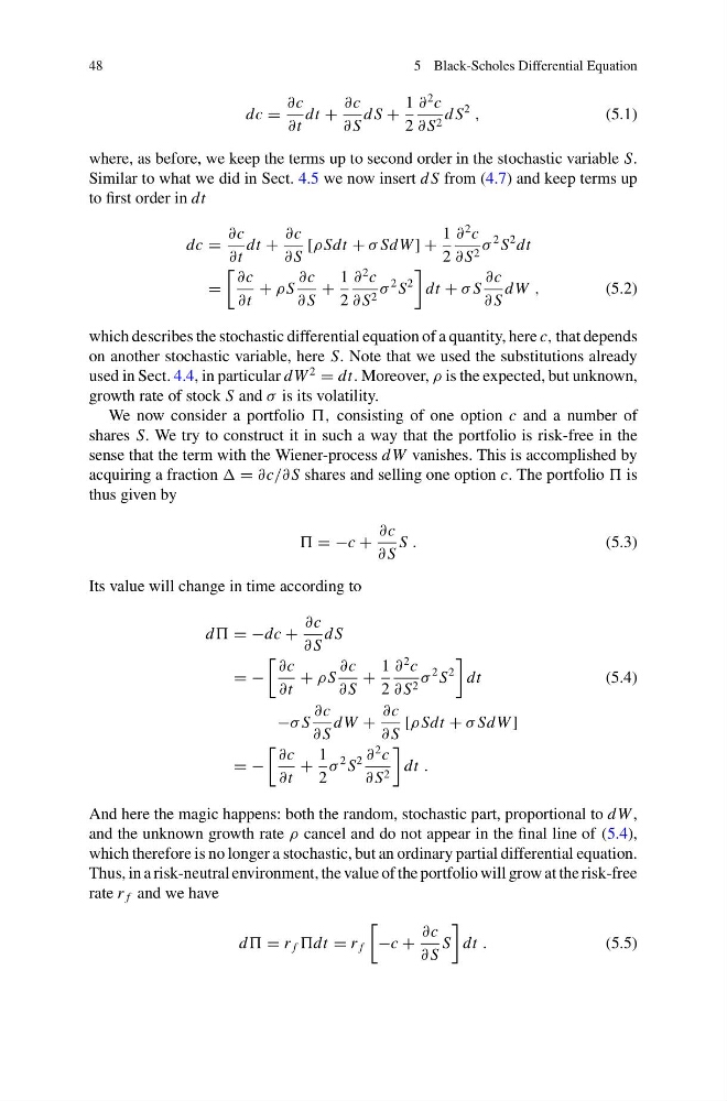
where, as before, we keep the terms up to second order in the stochastic variable S.
Similar to what we did in Sect. 4.5 we now insert d S from (4.7) and keep terms up
to first order in dt
dc =
∂c
∂t
dt +
∂c
∂ S
[ρ Sdt + σ SdW ] +
1
2
∂
2 c
∂ S 2 σ
2 S
2 dt
=
∂c
∂t
+ ρ S
∂c
∂ S
+
1
2
∂
2 c
∂ S 2 σ
2 S
2
dt + σ S
∂c
∂ S
dW ,
(5.2)
which describes the stochastic differential equation of a quantity, here c, that depends
on another stochastic variable, here S. Note that we used the substitutions already
used in Sect. 4.4, in particular dW
2
= dt. Moreover, ρ is the expected, but unknown,
growth rate of stock S and σ is its volatility.
We now consider a portfolio , consisting of one option c and a number of
shares S. We try to construct it in such a way that the portfolio is risk-free in the
sense that the term with the Wiener-process dW vanishes. This is accomplished by
acquiring a fraction = ∂c/∂ S shares and selling one option c. The portfolio is
thus given by
= −c +
∂c
∂ S
S .
(5.3)
Its value will change in time according to
d = −dc +
∂c
∂ S
d S
= −
∂c
∂t
+ ρ S
∂c
∂ S
+
1
2
∂
2 c
∂ S 2 σ
2 S
2
dt
(5.4)
−σ S
∂c
∂ S
dW +
∂c
∂ S
[ρ Sdt + σ SdW ]
= −
∂c
∂t
+
1
2
σ
2 S
2 ∂
2 c
∂ S 2
dt .
And here the magic happens: both the random, stochastic part, proportional to dW ,
and the unknown growth rate ρ cancel and do not appear in the final line of (5.4),
which therefore is no longer a stochastic, but an ordinary partial differential equation.
Thus, in a risk-neutral environment, the value of the portfolio will grow at the risk-free
rate r f and we have
d = r f dt = r f
−c +
∂c
∂ S
S
dt .
(5.5)
5 Black-Scholes Differential Equation
dc =
∂c
∂t
dt +
∂c
∂ S
d S +
1
2
∂
2 c
∂ S 2 d S
2
,
(5.1)
where, as before, we keep the terms up to second order in the stochastic variable S.
Similar to what we did in Sect. 4.5 we now insert d S from (4.7) and keep terms up
to first order in dt
dc =
∂c
∂t
dt +
∂c
∂ S
[ρ Sdt + σ SdW ] +
1
2
∂
2 c
∂ S 2 σ
2 S
2 dt
=
∂c
∂t
+ ρ S
∂c
∂ S
+
1
2
∂
2 c
∂ S 2 σ
2 S
2
dt + σ S
∂c
∂ S
dW ,
(5.2)
which describes the stochastic differential equation of a quantity, here c, that depends
on another stochastic variable, here S. Note that we used the substitutions already
used in Sect. 4.4, in particular dW
2
= dt. Moreover, ρ is the expected, but unknown,
growth rate of stock S and σ is its volatility.
We now consider a portfolio , consisting of one option c and a number of
shares S. We try to construct it in such a way that the portfolio is risk-free in the
sense that the term with the Wiener-process dW vanishes. This is accomplished by
acquiring a fraction = ∂c/∂ S shares and selling one option c. The portfolio is
thus given by
= −c +
∂c
∂ S
S .
(5.3)
Its value will change in time according to
d = −dc +
∂c
∂ S
d S
= −
∂c
∂t
+ ρ S
∂c
∂ S
+
1
2
∂
2 c
∂ S 2 σ
2 S
2
dt
(5.4)
−σ S
∂c
∂ S
dW +
∂c
∂ S
[ρ Sdt + σ SdW ]
= −
∂c
∂t
+
1
2
σ
2 S
2 ∂
2 c
∂ S 2
dt .
And here the magic happens: both the random, stochastic part, proportional to dW ,
and the unknown growth rate ρ cancel and do not appear in the final line of (5.4),
which therefore is no longer a stochastic, but an ordinary partial differential equation.
Thus, in a risk-neutral environment, the value of the portfolio will grow at the risk-free
rate r f and we have
d = r f dt = r f
−c +
∂c
∂ S
S
dt .
(5.5)