

4.2 Wiener Process
33
x(t n ) = 0
(4.11)
x(t n )
2
= σ
2
n
i=1
n
j=1
ξ(t i )ξ(t j ) = σ
2
n
i=1
n
j=1
δ i j = nσ
2
= t n
σ
2
t
.
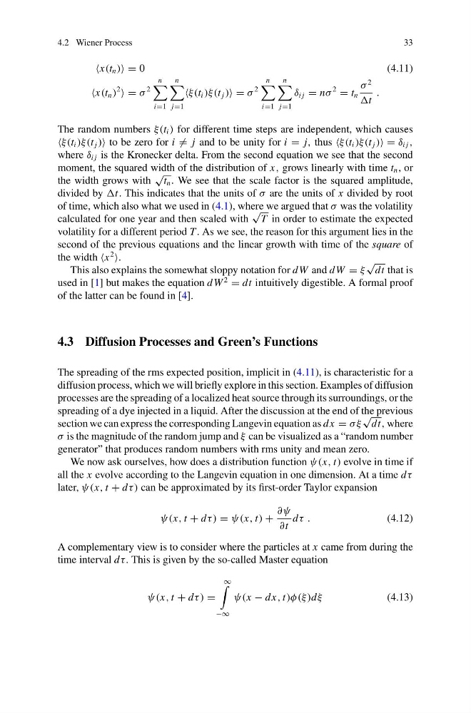
The random numbers ξ(t i ) for different time steps are independent, which causes
ξ(t i )ξ(t j ) to be zero for i = j and to be unity for i = j, thus ξ(t i )ξ(t j ) = δ i j ,
where δ i j is the Kronecker delta. From the second equation we see that the second
moment, the squared width of the distribution of x, grows linearly with time t n , or
the width grows with
√
t n . We see that the scale factor is the squared amplitude,
divided by t. This indicates that the units of σ are the units of x divided by root
of time, which also what we used in (4.1), where we argued that σ was the volatility
calculated for one year and then scaled with
√
T in order to estimate the expected
volatility for a different period T. As we see, the reason for this argument lies in the
second of the previous equations and the linear growth with time of the square of
the width x
2
.
This also explains the somewhat sloppy notation for dW and dW = ξ
√
dt that is
used in [1] but makes the equation dW
2
= dt intuitively digestible. A formal proof
of the latter can be found in [4].
4.3 Diffusion Processes and Green’s Functions
The spreading of the rms expected position, implicit in (4.11), is characteristic for a
diffusion process, which we will briefly explore in this section. Examples of diffusion
processes are the spreading of a localized heat source through its surroundings, or the
spreading of a dye injected in a liquid. After the discussion at the end of the previous
section we can express the corresponding Langevin equation as dx = σ ξ
√
dt, where
σ is the magnitude of the random jump and ξ can be visualized as a “random number
generator” that produces random numbers with rms unity and mean zero.
We now ask ourselves, how does a distribution function ψ(x, t) evolve in time if
all the x evolve according to the Langevin equation in one dimension. At a time dτ
later, ψ(x, t + dτ ) can be approximated by its first-order Taylor expansion
ψ(x, t + dτ ) = ψ(x, t) +
∂ψ
∂t
dτ .
(4.12)
A complementary view is to consider where the particles at x came from during the
time interval dτ. This is given by the so-called Master equation
ψ(x, t + dτ ) =
∞
−∞
ψ(x − dx, t)φ(ξ )dξ
(4.13)
33
x(t n ) = 0
(4.11)
x(t n )
2
= σ
2
n
i=1
n
j=1
ξ(t i )ξ(t j ) = σ
2
n
i=1
n
j=1
δ i j = nσ
2
= t n
σ
2
t
.
The random numbers ξ(t i ) for different time steps are independent, which causes
ξ(t i )ξ(t j ) to be zero for i = j and to be unity for i = j, thus ξ(t i )ξ(t j ) = δ i j ,
where δ i j is the Kronecker delta. From the second equation we see that the second
moment, the squared width of the distribution of x, grows linearly with time t n , or
the width grows with
√
t n . We see that the scale factor is the squared amplitude,
divided by t. This indicates that the units of σ are the units of x divided by root
of time, which also what we used in (4.1), where we argued that σ was the volatility
calculated for one year and then scaled with
√
T in order to estimate the expected
volatility for a different period T. As we see, the reason for this argument lies in the
second of the previous equations and the linear growth with time of the square of
the width x
2
.
This also explains the somewhat sloppy notation for dW and dW = ξ
√
dt that is
used in [1] but makes the equation dW
2
= dt intuitively digestible. A formal proof
of the latter can be found in [4].
4.3 Diffusion Processes and Green’s Functions
The spreading of the rms expected position, implicit in (4.11), is characteristic for a
diffusion process, which we will briefly explore in this section. Examples of diffusion
processes are the spreading of a localized heat source through its surroundings, or the
spreading of a dye injected in a liquid. After the discussion at the end of the previous
section we can express the corresponding Langevin equation as dx = σ ξ
√
dt, where
σ is the magnitude of the random jump and ξ can be visualized as a “random number
generator” that produces random numbers with rms unity and mean zero.
We now ask ourselves, how does a distribution function ψ(x, t) evolve in time if
all the x evolve according to the Langevin equation in one dimension. At a time dτ
later, ψ(x, t + dτ ) can be approximated by its first-order Taylor expansion
ψ(x, t + dτ ) = ψ(x, t) +
∂ψ
∂t
dτ .
(4.12)
A complementary view is to consider where the particles at x came from during the
time interval dτ. This is given by the so-called Master equation
ψ(x, t + dτ ) =
∞
−∞
ψ(x − dx, t)φ(ξ )dξ
(4.13)