

3.6 Valuation
27
raw materials. At the present time these values are unknown and need to be estimated.
Big changes can be expected, if new production facilities are opened within the time
horizon Y.
The discount rate r that is used to calculate the discounted cash flow describes
the annual cost of sustaining the capital V in the company. Often the W ACC, the
weighted average cost of capital, is substituted for r . It is given by
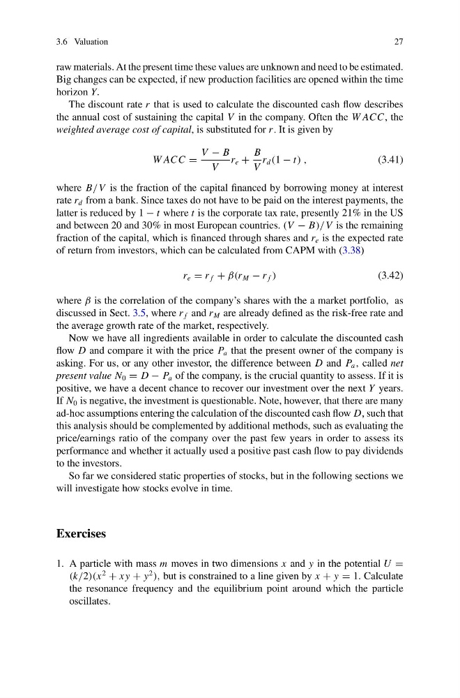
W ACC =
V − B
V
r e +
B
V
r d (1 − t) ,
(3.41)
where B/V is the fraction of the capital financed by borrowing money at interest
rate r d from a bank. Since taxes do not have to be paid on the interest payments, the
latter is reduced by 1 − t where t is the corporate tax rate, presently 21% in the US
and between 20 and 30% in most European countries. (V − B)/V is the remaining
fraction of the capital, which is financed through shares and r e is the expected rate
of return from investors, which can be calculated from CAPM with (3.38)
r e = r f + β(r M − r f )
(3.42)
where β is the correlation of the company’s shares with the a market portfolio, as
discussed in Sect. 3.5, where r f and r M are already defined as the risk-free rate and
the average growth rate of the market, respectively.
Now we have all ingredients available in order to calculate the discounted cash
flow D and compare it with the price P a that the present owner of the company is
asking. For us, or any other investor, the difference between D and P a , called net
present value N 0 = D − P a of the company, is the crucial quantity to assess. If it is
positive, we have a decent chance to recover our investment over the next Y years.
If N 0 is negative, the investment is questionable. Note, however, that there are many
ad-hoc assumptions entering the calculation of the discounted cash flow D, such that
this analysis should be complemented by additional methods, such as evaluating the
price/earnings ratio of the company over the past few years in order to assess its
performance and whether it actually used a positive past cash flow to pay dividends
to the investors.
So far we considered static properties of stocks, but in the following sections we
will investigate how stocks evolve in time.
Exercises
1. A particle with mass m moves in two dimensions x and y in the potential U =
(k/2)(x
2
+ x y + y
2
), but is constrained to a line given by x + y = 1. Calculate
the resonance frequency and the equilibrium point around which the particle
oscillates.
27
raw materials. At the present time these values are unknown and need to be estimated.
Big changes can be expected, if new production facilities are opened within the time
horizon Y.
The discount rate r that is used to calculate the discounted cash flow describes
the annual cost of sustaining the capital V in the company. Often the W ACC, the
weighted average cost of capital, is substituted for r . It is given by
W ACC =
V − B
V
r e +
B
V
r d (1 − t) ,
(3.41)
where B/V is the fraction of the capital financed by borrowing money at interest
rate r d from a bank. Since taxes do not have to be paid on the interest payments, the
latter is reduced by 1 − t where t is the corporate tax rate, presently 21% in the US
and between 20 and 30% in most European countries. (V − B)/V is the remaining
fraction of the capital, which is financed through shares and r e is the expected rate
of return from investors, which can be calculated from CAPM with (3.38)
r e = r f + β(r M − r f )
(3.42)
where β is the correlation of the company’s shares with the a market portfolio, as
discussed in Sect. 3.5, where r f and r M are already defined as the risk-free rate and
the average growth rate of the market, respectively.
Now we have all ingredients available in order to calculate the discounted cash
flow D and compare it with the price P a that the present owner of the company is
asking. For us, or any other investor, the difference between D and P a , called net
present value N 0 = D − P a of the company, is the crucial quantity to assess. If it is
positive, we have a decent chance to recover our investment over the next Y years.
If N 0 is negative, the investment is questionable. Note, however, that there are many
ad-hoc assumptions entering the calculation of the discounted cash flow D, such that
this analysis should be complemented by additional methods, such as evaluating the
price/earnings ratio of the company over the past few years in order to assess its
performance and whether it actually used a positive past cash flow to pay dividends
to the investors.
So far we considered static properties of stocks, but in the following sections we
will investigate how stocks evolve in time.
Exercises
1. A particle with mass m moves in two dimensions x and y in the potential U =
(k/2)(x
2
+ x y + y
2
), but is constrained to a line given by x + y = 1. Calculate
the resonance frequency and the equilibrium point around which the particle
oscillates.