

274
Appendix B: Software
B.6 Numerical Path Integrals
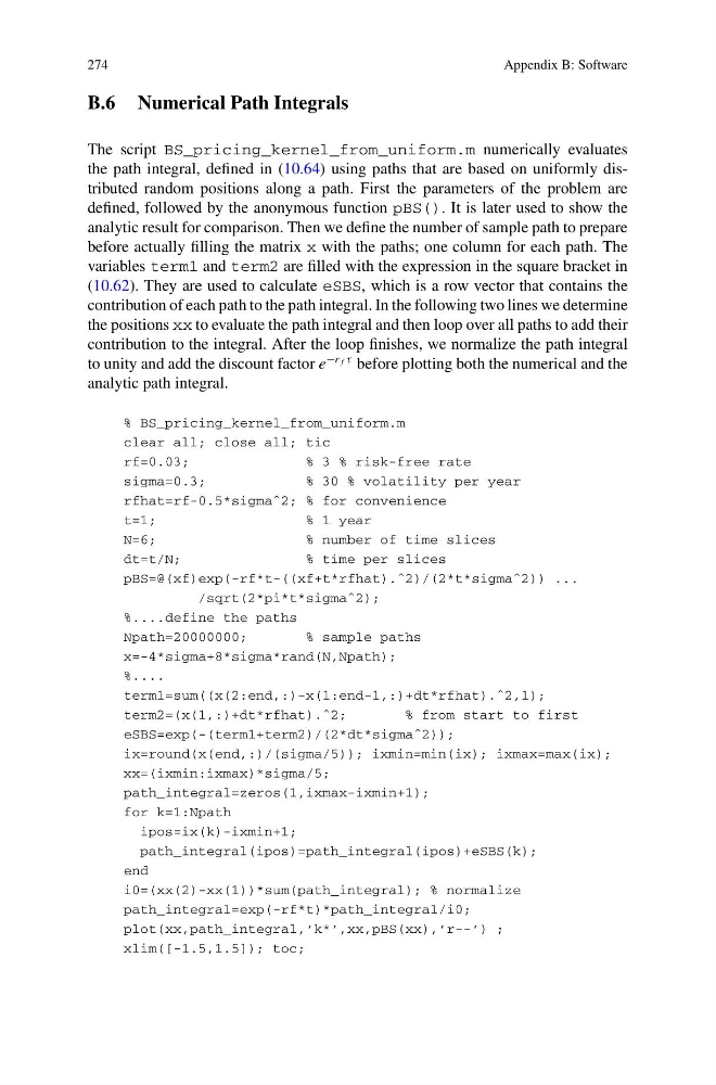
The script BS_pricing_kernel_from_uniform.m numerically evaluates
the path integral, defined in (10.64) using paths that are based on uniformly distributed random positions along a path. First the parameters of the problem are
defined, followed by the anonymous function pBS(). It is later used to show the
analytic result for comparison. Then we define the number of sample path to prepare
before actually filling the matrix x with the paths; one column for each path. The
variables term1 and term2 are filled with the expression in the square bracket in
(10.62). They are used to calculate eSBS, which is a row vector that contains the
contribution of each path to the path integral. In the following two lines we determine
the positions xx to evaluate the path integral and then loop over all paths to add their
contribution to the integral. After the loop finishes, we normalize the path integral
to unity and add the discount factor e
−r f τ before plotting both the numerical and the
analytic path integral.
% BS_pricing_kernel_from_uniform.m
clear all; close all; tic
rf=0.03;
% 3 % risk-free rate
sigma=0.3;
% 30 % volatility per year
rfhat=rf-0.5*sigmaˆ2; % for convenience
t=1;
% 1 year
N=6;
% number of time slices
dt=t/N;
% time per slices
pBS=@(xf)exp(-rf*t-((xf+t*rfhat).ˆ2)/(2*t*sigmaˆ2)) ...
/sqrt(2*pi*t*sigmaˆ2);
%....define the paths
Npath=20000000;
% sample paths
x=-4*sigma+8*sigma*rand(N,Npath);
%....
term1=sum((x(2:end,:)-x(1:end-1,:)+dt*rfhat).ˆ2,1);
term2=(x(1,:)+dt*rfhat).ˆ2;
% from start to first
eSBS=exp(-(term1+term2)/(2*dt*sigmaˆ2));
ix=round(x(end,:)/(sigma/5)); ixmin=min(ix); ixmax=max(ix);
xx=(ixmin:ixmax)*sigma/5;
path_integral=zeros(1,ixmax-ixmin+1);
for k=1:Npath
ipos=ix(k)-ixmin+1;
path_integral(ipos)=path_integral(ipos)+eSBS(k);
end
i0=(xx(2)-xx(1))*sum(path_integral); % normalize
path_integral=exp(-rf*t)*path_integral/i0;
plot(xx,path_integral,’k*’,xx,pBS(xx),’r--’) ;
xlim([-1.5,1.5]); toc;
Appendix B: Software
B.6 Numerical Path Integrals
The script BS_pricing_kernel_from_uniform.m numerically evaluates
the path integral, defined in (10.64) using paths that are based on uniformly distributed random positions along a path. First the parameters of the problem are
defined, followed by the anonymous function pBS(). It is later used to show the
analytic result for comparison. Then we define the number of sample path to prepare
before actually filling the matrix x with the paths; one column for each path. The
variables term1 and term2 are filled with the expression in the square bracket in
(10.62). They are used to calculate eSBS, which is a row vector that contains the
contribution of each path to the path integral. In the following two lines we determine
the positions xx to evaluate the path integral and then loop over all paths to add their
contribution to the integral. After the loop finishes, we normalize the path integral
to unity and add the discount factor e
−r f τ before plotting both the numerical and the
analytic path integral.
% BS_pricing_kernel_from_uniform.m
clear all; close all; tic
rf=0.03;
% 3 % risk-free rate
sigma=0.3;
% 30 % volatility per year
rfhat=rf-0.5*sigmaˆ2; % for convenience
t=1;
% 1 year
N=6;
% number of time slices
dt=t/N;
% time per slices
pBS=@(xf)exp(-rf*t-((xf+t*rfhat).ˆ2)/(2*t*sigmaˆ2)) ...
/sqrt(2*pi*t*sigmaˆ2);
%....define the paths
Npath=20000000;
% sample paths
x=-4*sigma+8*sigma*rand(N,Npath);
%....
term1=sum((x(2:end,:)-x(1:end-1,:)+dt*rfhat).ˆ2,1);
term2=(x(1,:)+dt*rfhat).ˆ2;
% from start to first
eSBS=exp(-(term1+term2)/(2*dt*sigmaˆ2));
ix=round(x(end,:)/(sigma/5)); ixmin=min(ix); ixmax=max(ix);
xx=(ixmin:ixmax)*sigma/5;
path_integral=zeros(1,ixmax-ixmin+1);
for k=1:Npath
ipos=ix(k)-ixmin+1;
path_integral(ipos)=path_integral(ipos)+eSBS(k);
end
i0=(xx(2)-xx(1))*sum(path_integral); % normalize
path_integral=exp(-rf*t)*path_integral/i0;
plot(xx,path_integral,’k*’,xx,pBS(xx),’r--’) ;
xlim([-1.5,1.5]); toc;