

Appendix B: Software
269
end
nn=1:N;
plot(nn,S,’b-’,nn,KK,’b:’,nn,hedge,’r’,nn,borrow,’g’);
xlim([0,255]); xlabel(’trading days’);
ylabel(’S,K,\Delta S,Borrowed’)
legend(’Stock S’,’Strike K’,’Hedge \Delta S’,’Borrowed’)
Once the loop completes, we test whether we have to deliver the share to the option
buyer and calculate our cost accordingly, before plotting the data and annotating the
axes.
B.4 Cantor, Koch, and Mandelbrot
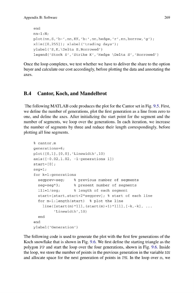
The following MATLAB code produces the plot for the Cantor set in Fig. 9.5. First,
we define the number of generations, plot the first generation as a line from zero to
one, and define the axes. After initializing the start point for the segment and the
number of segments, we loop over the generations. In each iteration, we increase
the number of segments by three and reduce their length correspondingly, before
plotting all line segments.
% cantor.m
generations=6;
plot([0,1],[0,0],’Linewidth’,10)
axis([-0.02,1.02, -1-generations 1])
start=[0];
seg=1;
for k=1:generations
segprev=seg;
% previous number of segments
seg=seg*3;
% present number of segments
lll=1/seg;
% length of each segment
start=[start,start+2*segprev]; % start of each line
for m=1:length(start) % plot the line
line([start(m)*lll,(start(m)+1)*lll],[-k,-k], ...
’Linewidth’,10)
end
end
ylabel(’Generation’)
The following code is used to generate the plot with the first few generations of the
Koch snowflake that is shown in Fig. 9.6. We first define the starting triangle as the
polygon PP and start the loop over the four generations, shown in Fig. 9.6. Inside
the loop, we store the number of points in the previous generation in the variable NN
and allocate space for the next generation of points in PN. In the loop over m, we
269
end
nn=1:N;
plot(nn,S,’b-’,nn,KK,’b:’,nn,hedge,’r’,nn,borrow,’g’);
xlim([0,255]); xlabel(’trading days’);
ylabel(’S,K,\Delta S,Borrowed’)
legend(’Stock S’,’Strike K’,’Hedge \Delta S’,’Borrowed’)
Once the loop completes, we test whether we have to deliver the share to the option
buyer and calculate our cost accordingly, before plotting the data and annotating the
axes.
B.4 Cantor, Koch, and Mandelbrot
The following MATLAB code produces the plot for the Cantor set in Fig. 9.5. First,
we define the number of generations, plot the first generation as a line from zero to
one, and define the axes. After initializing the start point for the segment and the
number of segments, we loop over the generations. In each iteration, we increase
the number of segments by three and reduce their length correspondingly, before
plotting all line segments.
% cantor.m
generations=6;
plot([0,1],[0,0],’Linewidth’,10)
axis([-0.02,1.02, -1-generations 1])
start=[0];
seg=1;
for k=1:generations
segprev=seg;
% previous number of segments
seg=seg*3;
% present number of segments
lll=1/seg;
% length of each segment
start=[start,start+2*segprev]; % start of each line
for m=1:length(start) % plot the line
line([start(m)*lll,(start(m)+1)*lll],[-k,-k], ...
’Linewidth’,10)
end
end
ylabel(’Generation’)
The following code is used to generate the plot with the first few generations of the
Koch snowflake that is shown in Fig. 9.6. We first define the starting triangle as the
polygon PP and start the loop over the four generations, shown in Fig. 9.6. Inside
the loop, we store the number of points in the previous generation in the variable NN
and allocate space for the next generation of points in PN. In the loop over m, we