

18
3 Portfolio Theory and CAPM
3.2 Portfolio with Risky Assets Only
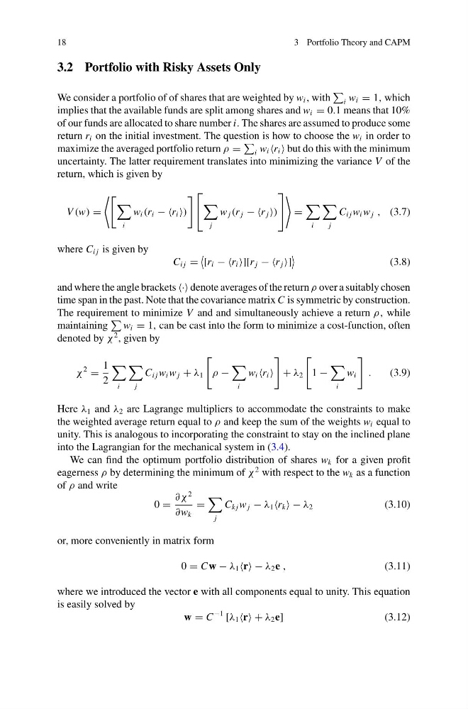
We consider a portfolio of of shares that are weighted by w i , with
i w i = 1, which
implies that the available funds are split among shares and w i = 0.1 means that 10%
of our funds are allocated to share number i. The shares are assumed to produce some
return r i on the initial investment. The question is how to choose the w i in order to
maximize the averaged portfolio return ρ =
i w i r i but do this with the minimum
uncertainty. The latter requirement translates into minimizing the variance V of the
return, which is given by
V (w) =
i
w i (r i − −r i )
⎡
⎣
j
w j (r j − −r j )
⎤
⎦
=
i
j
C i j w i w j , (3.7)
where C i j is given by
C i j =
[r i − −r i ][r j − −r j ]
(3.8)
and where the angle brackets ·· denote averages of the return ρ over a suitably chosen
time span in the past. Note that the covariance matrix C is symmetric by construction.
The requirement to minimize V and and simultaneously achieve a return ρ, while
maintaining
w i = 1, can be cast into the form to minimize a cost-function, often
denoted by χ
2 , given by
χ
2
=
1
2
i
j
C i j w i w j + λ 1
ρ −
i
w i r i
+ λ 2
1 −
i
w i
.
(3.9)
Here λ 1 and λ 2 are Lagrange multipliers to accommodate the constraints to make
the weighted average return equal to ρ and keep the sum of the weights w i equal to
unity. This is analogous to incorporating the constraint to stay on the inclined plane
into the Lagrangian for the mechanical system in (3.4).
We can find the optimum portfolio distribution of shares w k for a given profit
eagerness ρ by determining the minimum of χ
2 with respect to the w k as a function
of ρ and write
0 =
∂χ
2
∂w k
=
j
C k j w j − λ 1 r k − λ 2
(3.10)
or, more conveniently in matrix form
0 = Cw − λ 1 r − λ 2 e ,
(3.11)
where we introduced the vector e with all components equal to unity. This equation
is easily solved by
w = C
−1 [λ 1 r + λ 2 e]
(3.12)
3 Portfolio Theory and CAPM
3.2 Portfolio with Risky Assets Only
We consider a portfolio of of shares that are weighted by w i , with
i w i = 1, which
implies that the available funds are split among shares and w i = 0.1 means that 10%
of our funds are allocated to share number i. The shares are assumed to produce some
return r i on the initial investment. The question is how to choose the w i in order to
maximize the averaged portfolio return ρ =
i w i r i but do this with the minimum
uncertainty. The latter requirement translates into minimizing the variance V of the
return, which is given by
V (w) =
i
w i (r i − −r i )
⎡
⎣
j
w j (r j − −r j )
⎤
⎦
=
i
j
C i j w i w j , (3.7)
where C i j is given by
C i j =
[r i − −r i ][r j − −r j ]
(3.8)
and where the angle brackets ·· denote averages of the return ρ over a suitably chosen
time span in the past. Note that the covariance matrix C is symmetric by construction.
The requirement to minimize V and and simultaneously achieve a return ρ, while
maintaining
w i = 1, can be cast into the form to minimize a cost-function, often
denoted by χ
2 , given by
χ
2
=
1
2
i
j
C i j w i w j + λ 1
ρ −
i
w i r i
+ λ 2
1 −
i
w i
.
(3.9)
Here λ 1 and λ 2 are Lagrange multipliers to accommodate the constraints to make
the weighted average return equal to ρ and keep the sum of the weights w i equal to
unity. This is analogous to incorporating the constraint to stay on the inclined plane
into the Lagrangian for the mechanical system in (3.4).
We can find the optimum portfolio distribution of shares w k for a given profit
eagerness ρ by determining the minimum of χ
2 with respect to the w k as a function
of ρ and write
0 =
∂χ
2
∂w k
=
j
C k j w j − λ 1 r k − λ 2
(3.10)
or, more conveniently in matrix form
0 = Cw − λ 1 r − λ 2 e ,
(3.11)
where we introduced the vector e with all components equal to unity. This equation
is easily solved by
w = C
−1 [λ 1 r + λ 2 e]
(3.12)