

254
13 Solutions for Selected Exercises
cauchy=@(x)(1/pi)./(1+x.*x);
N=1000000; x0=1; beta=1;
y=metropolis3(cauchy,beta,1000,x0);
% burn in
x=metropolis3(cauchy,beta,N,y(1000));
dx=0.1; xx=-30:dx:30;
% for plotting
hist(x,xx); hold on; plot(xx,N*cauchy(xx)*dx,’r’)
Exercise 11.1
The full MATLAB code is available in the file ex11_1.m from the ESM. Varying
the investment fraction σ we find that the utility V [ p] has a maximum at about 2.78
for σ = 0.43.
Exercise 11.2
The following code snippet implements the recursion relation for the random process
λ. Plotting the values shows that they slowly approach a constant value.
lambda=zeros(1,n);
for t=2:n
lambda(t)=gamma*lambda(t-1)+(2-gamma)+a*randn;
end
The asymptotic value λ ∞ is determined by the condition λ ∞ = λ t+1 = λ t and replacing ε t by its average value, which is zero. The equation defining the stochastic process
λ then becomes λ ∞ = γ λ ∞ + (2 − γ ), which we solve for λ ∞ = (2 − γ )/(1 − γ ).
For γ = 0.9 we find λ ∞ = 11.
Exercise 11.3
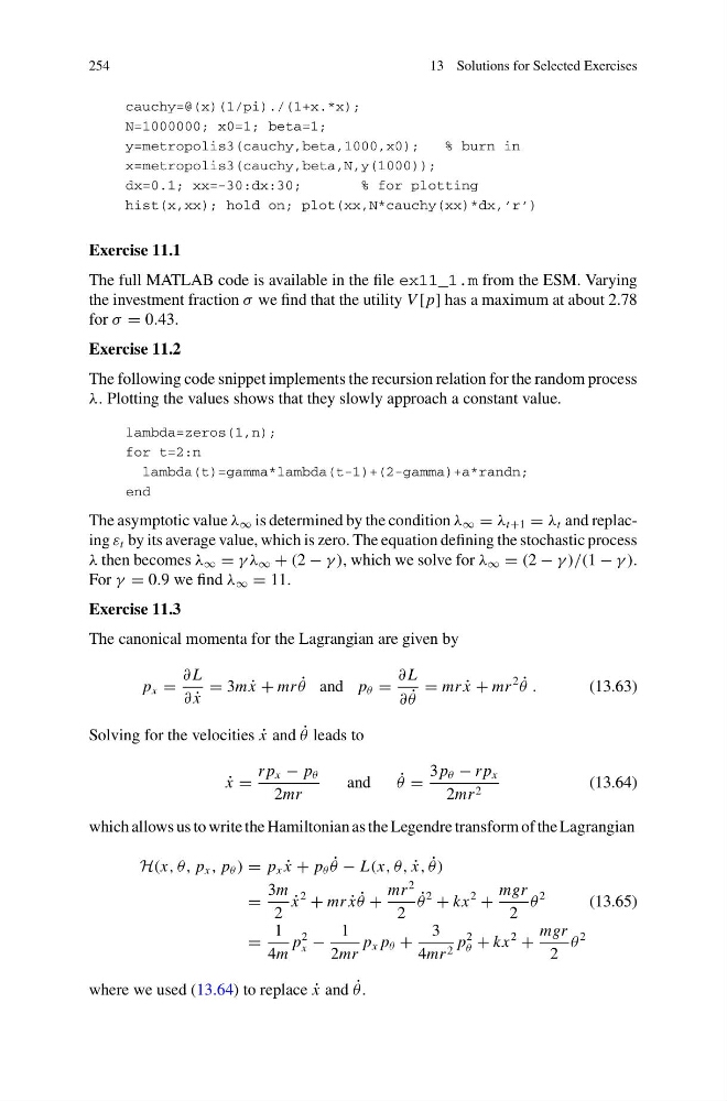
The canonical momenta for the Lagrangian are given by
p x =
∂ L
∂ ˙
x
= 3m ˙
x + mr ˙
θ and p θ =
∂ L
∂ ˙
θ
= mr ˙
x + mr
2 ˙
θ .
(13.63)
Solving for the velocities ˙
x and ˙
θ leads to
˙
x =
r p x − p θ
2mr
and
˙
θ =
3 p θ − r p x
2mr 2
(13.64)
which allows us to write the Hamiltonian as the Legendre transform of the Lagrangian
H(x, θ, p x , p θ ) = p x ˙
x + p θ ˙
θ − L(x, θ, ˙
x, ˙
θ)
=
3m
2
˙
x
2
+ mr ˙
x ˙
θ +
mr
2
2
˙
θ
2
+ kx
2
+
mgr
2
θ
2
(13.65)
=
1
4m
p
2
x −
1
2mr
p x p θ +
3
4mr 2 p
2
θ + kx
2
+
mgr
2
θ
2
where we used (13.64) to replace ˙
x and ˙
θ .
13 Solutions for Selected Exercises
cauchy=@(x)(1/pi)./(1+x.*x);
N=1000000; x0=1; beta=1;
y=metropolis3(cauchy,beta,1000,x0);
% burn in
x=metropolis3(cauchy,beta,N,y(1000));
dx=0.1; xx=-30:dx:30;
% for plotting
hist(x,xx); hold on; plot(xx,N*cauchy(xx)*dx,’r’)
Exercise 11.1
The full MATLAB code is available in the file ex11_1.m from the ESM. Varying
the investment fraction σ we find that the utility V [ p] has a maximum at about 2.78
for σ = 0.43.
Exercise 11.2
The following code snippet implements the recursion relation for the random process
λ. Plotting the values shows that they slowly approach a constant value.
lambda=zeros(1,n);
for t=2:n
lambda(t)=gamma*lambda(t-1)+(2-gamma)+a*randn;
end
The asymptotic value λ ∞ is determined by the condition λ ∞ = λ t+1 = λ t and replacing ε t by its average value, which is zero. The equation defining the stochastic process
λ then becomes λ ∞ = γ λ ∞ + (2 − γ ), which we solve for λ ∞ = (2 − γ )/(1 − γ ).
For γ = 0.9 we find λ ∞ = 11.
Exercise 11.3
The canonical momenta for the Lagrangian are given by
p x =
∂ L
∂ ˙
x
= 3m ˙
x + mr ˙
θ and p θ =
∂ L
∂ ˙
θ
= mr ˙
x + mr
2 ˙
θ .
(13.63)
Solving for the velocities ˙
x and ˙
θ leads to
˙
x =
r p x − p θ
2mr
and
˙
θ =
3 p θ − r p x
2mr 2
(13.64)
which allows us to write the Hamiltonian as the Legendre transform of the Lagrangian
H(x, θ, p x , p θ ) = p x ˙
x + p θ ˙
θ − L(x, θ, ˙
x, ˙
θ)
=
3m
2
˙
x
2
+ mr ˙
x ˙
θ +
mr
2
2
˙
θ
2
+ kx
2
+
mgr
2
θ
2
(13.65)
=
1
4m
p
2
x −
1
2mr
p x p θ +
3
4mr 2 p
2
θ + kx
2
+
mgr
2
θ
2
where we used (13.64) to replace ˙
x and ˙
θ .