

13 Solutions for Selected Exercises
249
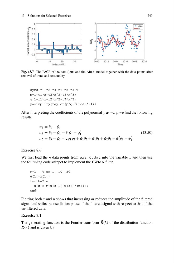
Fig. 13.7 The PACF of the data (left) and the AR(2)-model together with the data points after
removal of trend and seasonality
syms f1 f2 f3 t1 t2 t3 x
p=1-t1*x-t2*xˆ2-t3*xˆ3;
q=1-f1*x-f2*xˆ2-f3*xˆ3;
y=simplify(taylor(p/q,’Order’,4))
After interpreting the coefficients of the polynomial y as −π j , we find the following
results
π 1 = θ 1 − φ 1
π 2 = θ 2 − φ 2 + θ 1 φ 1 − φ
2
1
(13.50)
π 3 = θ 3 − φ 3 − 2φ 1 φ 2 + φ 1 θ 2 + φ 1 θ 2 + φ 2 θ 1 + φ
2
1 θ 1 − φ
3
1 .
Exercise 8.6
We first load the n data points from ex8_6.dat into the variable x and then use
the following code snippet to implement the EWMA filter.
m=3
% or 1, 10, 30
u(1)=x(1);
for k=2:n
u(k)=(m*u(k-1)+x(k))/(m+1);
end
Plotting both x and u shows that increasing m reduces the amplitude of the filtered
signal and shifts the oscillation phase of the filtered signal with respect to that of the
un-filtered data.
Exercise 9.1
The generating function is the Fourier transform ˜
R(k) of the distribution function
R(x) and is given by
249
Fig. 13.7 The PACF of the data (left) and the AR(2)-model together with the data points after
removal of trend and seasonality
syms f1 f2 f3 t1 t2 t3 x
p=1-t1*x-t2*xˆ2-t3*xˆ3;
q=1-f1*x-f2*xˆ2-f3*xˆ3;
y=simplify(taylor(p/q,’Order’,4))
After interpreting the coefficients of the polynomial y as −π j , we find the following
results
π 1 = θ 1 − φ 1
π 2 = θ 2 − φ 2 + θ 1 φ 1 − φ
2
1
(13.50)
π 3 = θ 3 − φ 3 − 2φ 1 φ 2 + φ 1 θ 2 + φ 1 θ 2 + φ 2 θ 1 + φ
2
1 θ 1 − φ
3
1 .
Exercise 8.6
We first load the n data points from ex8_6.dat into the variable x and then use
the following code snippet to implement the EWMA filter.
m=3
% or 1, 10, 30
u(1)=x(1);
for k=2:n
u(k)=(m*u(k-1)+x(k))/(m+1);
end
Plotting both x and u shows that increasing m reduces the amplitude of the filtered
signal and shifts the oscillation phase of the filtered signal with respect to that of the
un-filtered data.
Exercise 9.1
The generating function is the Fourier transform ˜
R(k) of the distribution function
R(x) and is given by