

16
3 Portfolio Theory and CAPM
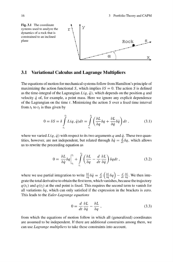
Fig. 3.1 The coordinate
systems used to analyze the
dynamics of a rock that is
constrained to an inclined
plane
3.1 Variational Calculus and Lagrange Multipliers
The equations of motion for mechanical systems follow from Hamilton’s principle of
maximizing the action functional S, which implies δS = 0. The action S is defined
as the time-integral of the Lagrangian L(q, ˙
q), which depends on the position q and
velocity ˙
q of, for example, a point mass. Here we ignore any explicit dependence
of the Lagrangian on the time t. Minimizing the action S over a fixed time interval
from t 1 to t 2 is thus given by
0 = δS = δ
t 2
t 1
L(q, ˙
q)dt =
t 2
t 1
∂ L
∂q
δq +
∂ L
∂ ˙
q
δ ˙
q
dt ,
(3.1)
where we varied L(q, ˙
q) with respect to its two arguments q and ˙
q. These two quantities, however, are not independent, but related through δ ˙
q =
d
dt
δq, which allows
us to rewrite the preceeding equation as
0 =
∂ L
∂ ˙
q
δq
t 2
t 1
+
t 2
t 1
∂ L
∂q
−
d
dt
∂ L
∂ ˙
q
δqdt ,
(3.2)
where we use partial integration to write
∂ L
∂ ˙
q
δ ˙
q =
d
dt
∂ L
∂ ˙
q
δq
−
d
dt
∂ L
∂ ˙
q
. We then integrate the total derivative to obtain the first term, which vanishes, because the trajectory
q(t 1 ) and q(t 2 ) at the end point is fixed. This requires the second term to vanish for
all variations δq, which can only satisfied if the expression in the brackets is zero.
This leads to the Euler-Lagrange equations
0 =
d
dt
∂ L
∂ ˙
q
−
∂ L
∂q
,
(3.3)
from which the equations of motion follow in which all (generalized) coordinates
are assumed to be independent. If there are additional constraints among them, we
can use Lagrange multipliers to take these constraints into account.
3 Portfolio Theory and CAPM
Fig. 3.1 The coordinate
systems used to analyze the
dynamics of a rock that is
constrained to an inclined
plane
3.1 Variational Calculus and Lagrange Multipliers
The equations of motion for mechanical systems follow from Hamilton’s principle of
maximizing the action functional S, which implies δS = 0. The action S is defined
as the time-integral of the Lagrangian L(q, ˙
q), which depends on the position q and
velocity ˙
q of, for example, a point mass. Here we ignore any explicit dependence
of the Lagrangian on the time t. Minimizing the action S over a fixed time interval
from t 1 to t 2 is thus given by
0 = δS = δ
t 2
t 1
L(q, ˙
q)dt =
t 2
t 1
∂ L
∂q
δq +
∂ L
∂ ˙
q
δ ˙
q
dt ,
(3.1)
where we varied L(q, ˙
q) with respect to its two arguments q and ˙
q. These two quantities, however, are not independent, but related through δ ˙
q =
d
dt
δq, which allows
us to rewrite the preceeding equation as
0 =
∂ L
∂ ˙
q
δq
t 2
t 1
+
t 2
t 1
∂ L
∂q
−
d
dt
∂ L
∂ ˙
q
δqdt ,
(3.2)
where we use partial integration to write
∂ L
∂ ˙
q
δ ˙
q =
d
dt
∂ L
∂ ˙
q
δq
−
d
dt
∂ L
∂ ˙
q
. We then integrate the total derivative to obtain the first term, which vanishes, because the trajectory
q(t 1 ) and q(t 2 ) at the end point is fixed. This requires the second term to vanish for
all variations δq, which can only satisfied if the expression in the brackets is zero.
This leads to the Euler-Lagrange equations
0 =
d
dt
∂ L
∂ ˙
q
−
∂ L
∂q
,
(3.3)
from which the equations of motion follow in which all (generalized) coordinates
are assumed to be independent. If there are additional constraints among them, we
can use Lagrange multipliers to take these constraints into account.