

11.4 Hamiltonians for Optimal Control
183
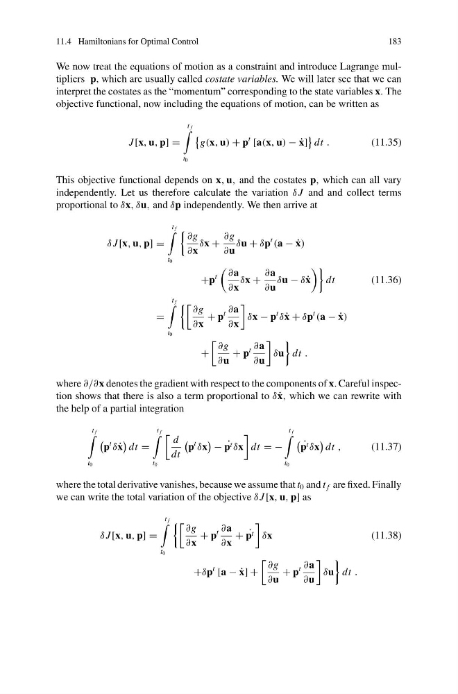
We now treat the equations of motion as a constraint and introduce Lagrange multipliers p, which are usually called costate variables. We will later see that we can
interpret the costates as the “momentum” corresponding to the state variables x. The
objective functional, now including the equations of motion, can be written as
J [x, u, p] =
t f
t 0
g(x, u) + p
t [a(x, u) − ˙
x]
dt .
(11.35)
This objective functional depends on x, u, and the costates p, which can all vary
independently. Let us therefore calculate the variation δ J and and collect terms
proportional to δx, δu, and δp independently. We then arrive at
δ J [x, u, p] =
t f
t 0
∂g
∂x
δx +
∂g
∂u
δu + δp
t
(a − ˙
x)
+p
t
∂a
∂x
δx +
∂a
∂u
δu − δ ˙
x
dt
(11.36)
=
t f
t 0
∂g
∂x
+ p
t ∂a
∂x
δx − p
t
δ ˙
x + δp
t
(a − ˙
x)
+
∂g
∂u
+ p
t ∂a
∂u
δu
dt .
where ∂/∂x denotes the gradient with respect to the components of x. Careful inspection shows that there is also a term proportional to δ ˙
x, which we can rewrite with
the help of a partial integration
t f
t 0
p
t
δ ˙
x
dt =
t f
t 0
d
dt
p
t
δx
− ˙
p t δx
dt = −
t f
t 0
˙
p t δx
dt ,
(11.37)
where the total derivative vanishes, because we assume that t 0 and t f are fixed. Finally
we can write the total variation of the objective δ J [x, u, p] as
δ J [x, u, p] =
t f
t 0
∂g
∂x
+ p
t ∂a
∂x
+ ˙
p t
δx
(11.38)
+δp
t [a − ˙
x] +
∂g
∂u
+ p
t ∂a
∂u
δu
dt .
183
We now treat the equations of motion as a constraint and introduce Lagrange multipliers p, which are usually called costate variables. We will later see that we can
interpret the costates as the “momentum” corresponding to the state variables x. The
objective functional, now including the equations of motion, can be written as
J [x, u, p] =
t f
t 0
g(x, u) + p
t [a(x, u) − ˙
x]
dt .
(11.35)
This objective functional depends on x, u, and the costates p, which can all vary
independently. Let us therefore calculate the variation δ J and and collect terms
proportional to δx, δu, and δp independently. We then arrive at
δ J [x, u, p] =
t f
t 0
∂g
∂x
δx +
∂g
∂u
δu + δp
t
(a − ˙
x)
+p
t
∂a
∂x
δx +
∂a
∂u
δu − δ ˙
x
dt
(11.36)
=
t f
t 0
∂g
∂x
+ p
t ∂a
∂x
δx − p
t
δ ˙
x + δp
t
(a − ˙
x)
+
∂g
∂u
+ p
t ∂a
∂u
δu
dt .
where ∂/∂x denotes the gradient with respect to the components of x. Careful inspection shows that there is also a term proportional to δ ˙
x, which we can rewrite with
the help of a partial integration
t f
t 0
p
t
δ ˙
x
dt =
t f
t 0
d
dt
p
t
δx
− ˙
p t δx
dt = −
t f
t 0
˙
p t δx
dt ,
(11.37)
where the total derivative vanishes, because we assume that t 0 and t f are fixed. Finally
we can write the total variation of the objective δ J [x, u, p] as
δ J [x, u, p] =
t f
t 0
∂g
∂x
+ p
t ∂a
∂x
+ ˙
p t
δx
(11.38)
+δp
t [a − ˙
x] +
∂g
∂u
+ p
t ∂a
∂u
δu
dt .