

176
11 Optimal Control Theory
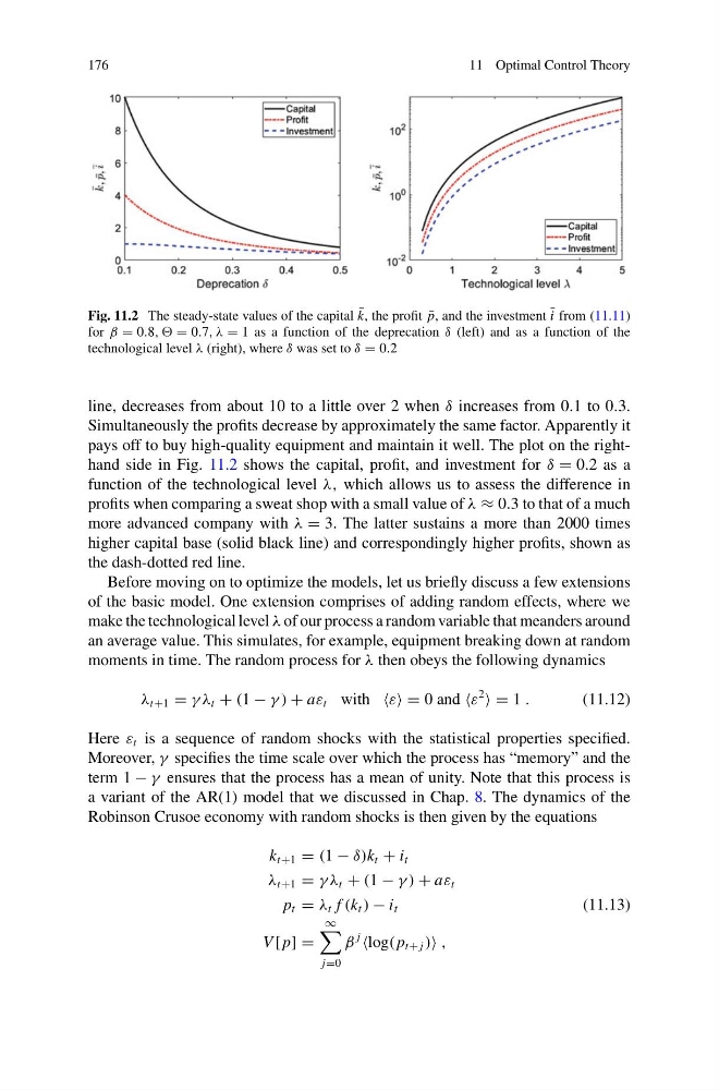
Fig. 11.2 The steady-state values of the capital ¯
k, the profit ¯
p, and the investment ¯
i from (11.11)
for β = 0.8, , = 0.7, λ = 1 as a function of the deprecation δ (left) and as a function of the
technological level λ (right), where δ was set to δ = 0.2
line, decreases from about 10 to a little over 2 when δ increases from 0.1 to 0.3.
Simultaneously the profits decrease by approximately the same factor. Apparently it
pays off to buy high-quality equipment and maintain it well. The plot on the righthand side in Fig. 11.2 shows the capital, profit, and investment for δ = 0.2 as a
function of the technological level λ, which allows us to assess the difference in
profits when comparing a sweat shop with a small value of λ ≈ 0.3 to that of a much
more advanced company with λ = 3. The latter sustains a more than 2000 times
higher capital base (solid black line) and correspondingly higher profits, shown as
the dash-dotted red line.
Before moving on to optimize the models, let us briefly discuss a few extensions
of the basic model. One extension comprises of adding random effects, where we
make the technological level λ of our process a random variable that meanders around
an average value. This simulates, for example, equipment breaking down at random
moments in time. The random process for λ then obeys the following dynamics
λ t+1 = γ λ t + (1 − γ ) + aε t with ε = 0 and ε
2
= 1 .
(11.12)
Here ε t is a sequence of random shocks with the statistical properties specified.
Moreover, γ specifies the time scale over which the process has “memory” and the
term 1 − γ ensures that the process has a mean of unity. Note that this process is
a variant of the AR(1) model that we discussed in Chap. 8. The dynamics of the
Robinson Crusoe economy with random shocks is then given by the equations
k t+1 = (1 − δ)k t + i t
λ t+1 = γ λ t + (1 − γ ) + aε t
p t = λ t f (k t ) − i t
(11.13)
V [ p] =
∞
j=0
β
j
log( p t+ j ) ,
11 Optimal Control Theory
Fig. 11.2 The steady-state values of the capital ¯
k, the profit ¯
p, and the investment ¯
i from (11.11)
for β = 0.8, , = 0.7, λ = 1 as a function of the deprecation δ (left) and as a function of the
technological level λ (right), where δ was set to δ = 0.2
line, decreases from about 10 to a little over 2 when δ increases from 0.1 to 0.3.
Simultaneously the profits decrease by approximately the same factor. Apparently it
pays off to buy high-quality equipment and maintain it well. The plot on the righthand side in Fig. 11.2 shows the capital, profit, and investment for δ = 0.2 as a
function of the technological level λ, which allows us to assess the difference in
profits when comparing a sweat shop with a small value of λ ≈ 0.3 to that of a much
more advanced company with λ = 3. The latter sustains a more than 2000 times
higher capital base (solid black line) and correspondingly higher profits, shown as
the dash-dotted red line.
Before moving on to optimize the models, let us briefly discuss a few extensions
of the basic model. One extension comprises of adding random effects, where we
make the technological level λ of our process a random variable that meanders around
an average value. This simulates, for example, equipment breaking down at random
moments in time. The random process for λ then obeys the following dynamics
λ t+1 = γ λ t + (1 − γ ) + aε t with ε = 0 and ε
2
= 1 .
(11.12)
Here ε t is a sequence of random shocks with the statistical properties specified.
Moreover, γ specifies the time scale over which the process has “memory” and the
term 1 − γ ensures that the process has a mean of unity. Note that this process is
a variant of the AR(1) model that we discussed in Chap. 8. The dynamics of the
Robinson Crusoe economy with random shocks is then given by the equations
k t+1 = (1 − δ)k t + i t
λ t+1 = γ λ t + (1 − γ ) + aε t
p t = λ t f (k t ) − i t
(11.13)
V [ p] =
∞
j=0
β
j
log( p t+ j ) ,