

10.5 Path Integrals in Quantum Mechanics
157
where L(x, ˙
x) = m ˙
x
2
/2 − V (x) is the Lagrange function that characterizes the
dynamics of the system. Here we only consider Lagrangians without explicit timedependence. The weight assigned to each path is e
i S(b,a)/
, such that we express the
propagator K (x b , t b ; x a , t a ) as
K (x b , t b ; x a , t a ) ∝
all paths
e
i S(b,a)/
,
(10.44)
which means that each path from a to b is weighted by a phase factor that depends
on the action S(b, a) on that path. Since we are dealing with quantum mechanical
systems, we divide the action S(b, a) by , which has the same units (Joule-seconds)
as the action and therefore makes the exponent dimensionless.
Owing to the smallness of the value of S/ varies a lot and contributions
of different paths interfere destructively, unless many paths in the vicinity have
similar values of the action S(b, a). But this happens near a path ¯
x(t) for which the
action S(b, a) is stationary when varying that path a little bit, or δS = 0. But this
requirement for stationarity is just Hamilton’s principle, which we know leads to the
Euler-Lagrange equations for the equations of motion that determine the trajectory
¯
x of the equivalent classical system. This means that the paths near the solution ¯
x
of the equations of motion for the classical system contribute most to the propagator
K , all the others paths will interfere destructively and average out.
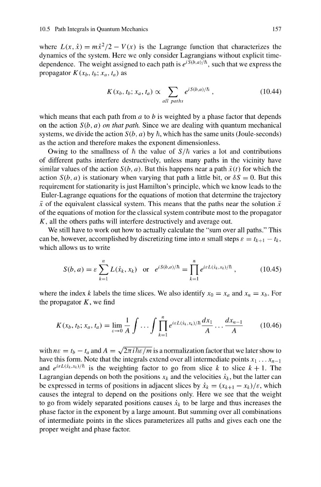
We still have to work out how to actually calculate the “sum over all paths.” This
can be, however, accomplished by discretizing time into n small steps ε = t k+1 − t k ,
which allows us to write
S(b, a) = ε
n
k=1
L( ˙
x k , x k ) or e
i S(b,a)/
=
n
k=1
e
iεL( ˙
x k ,x k )/
,
(10.45)
where the index k labels the time slices. We also identify x 0 = x a and x n = x b . For
the propagator K , we find
K (x b , t b ; x a , t a ) = lim
ε→0
1
A
. . .
n
k=1
e
iεL( ˙
x k ,x k )/ dx 1
A
. . .
dx n−1
A
(10.46)
with nε = t b − t a and A =
√
2πiε/m is a normalization factor that we later show to
have this form. Note that the integrals extend over all intermediate points x 1 . . . x n−1
and e
iεL( ˙
x k ,x k )/ is the weighting factor to go from slice k to slice k + 1. The
Lagrangian depends on both the positions x k and the velocities ˙
x k , but the latter can
be expressed in terms of positions in adjacent slices by ˙
x k = (x k+1 − x k )/ε, which
causes the integral to depend on the positions only. Here we see that the weight
to go from widely separated positions causes ˙
x k to be large and thus increases the
phase factor in the exponent by a large amount. But summing over all combinations
of intermediate points in the slices parameterizes all paths and gives each one the
proper weight and phase factor.
157
where L(x, ˙
x) = m ˙
x
2
/2 − V (x) is the Lagrange function that characterizes the
dynamics of the system. Here we only consider Lagrangians without explicit timedependence. The weight assigned to each path is e
i S(b,a)/
, such that we express the
propagator K (x b , t b ; x a , t a ) as
K (x b , t b ; x a , t a ) ∝
all paths
e
i S(b,a)/
,
(10.44)
which means that each path from a to b is weighted by a phase factor that depends
on the action S(b, a) on that path. Since we are dealing with quantum mechanical
systems, we divide the action S(b, a) by , which has the same units (Joule-seconds)
as the action and therefore makes the exponent dimensionless.
Owing to the smallness of the value of S/ varies a lot and contributions
of different paths interfere destructively, unless many paths in the vicinity have
similar values of the action S(b, a). But this happens near a path ¯
x(t) for which the
action S(b, a) is stationary when varying that path a little bit, or δS = 0. But this
requirement for stationarity is just Hamilton’s principle, which we know leads to the
Euler-Lagrange equations for the equations of motion that determine the trajectory
¯
x of the equivalent classical system. This means that the paths near the solution ¯
x
of the equations of motion for the classical system contribute most to the propagator
K , all the others paths will interfere destructively and average out.
We still have to work out how to actually calculate the “sum over all paths.” This
can be, however, accomplished by discretizing time into n small steps ε = t k+1 − t k ,
which allows us to write
S(b, a) = ε
n
k=1
L( ˙
x k , x k ) or e
i S(b,a)/
=
n
k=1
e
iεL( ˙
x k ,x k )/
,
(10.45)
where the index k labels the time slices. We also identify x 0 = x a and x n = x b . For
the propagator K , we find
K (x b , t b ; x a , t a ) = lim
ε→0
1
A
. . .
n
k=1
e
iεL( ˙
x k ,x k )/ dx 1
A
. . .
dx n−1
A
(10.46)
with nε = t b − t a and A =
√
2πiε/m is a normalization factor that we later show to
have this form. Note that the integrals extend over all intermediate points x 1 . . . x n−1
and e
iεL( ˙
x k ,x k )/ is the weighting factor to go from slice k to slice k + 1. The
Lagrangian depends on both the positions x k and the velocities ˙
x k , but the latter can
be expressed in terms of positions in adjacent slices by ˙
x k = (x k+1 − x k )/ε, which
causes the integral to depend on the positions only. Here we see that the weight
to go from widely separated positions causes ˙
x k to be large and thus increases the
phase factor in the exponent by a large amount. But summing over all combinations
of intermediate points in the slices parameterizes all paths and gives each one the
proper weight and phase factor.