

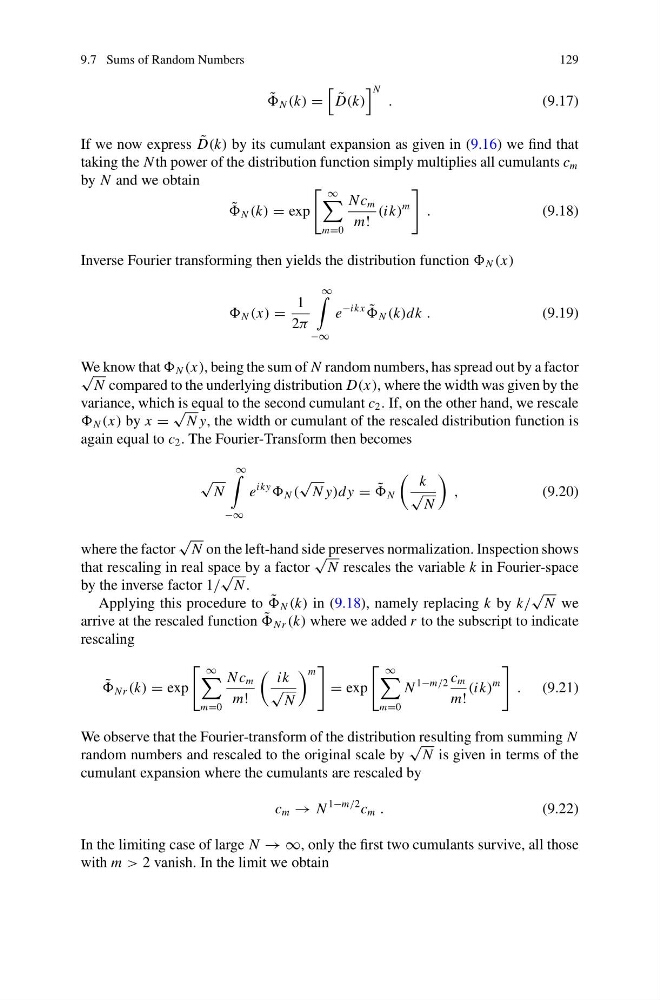
9.7 Sums of Random Numbers
129
˜
N (k) =
˜
D(k)
N .
(9.17)
If we now express ˜
D(k) by its cumulant expansion as given in (9.16) we find that
taking the N th power of the distribution function simply multiplies all cumulants c m
by N and we obtain
˜
N (k) = exp
∞
m=0
N c m
m!
(ik)
m
.
(9.18)
Inverse Fourier transforming then yields the distribution function N (x)
N (x) =
1
2π
∞
−∞
e
−ikx ˜
N (k)dk .
(9.19)
We know that N (x), being the sum of N random numbers, has spread out by a factor
√
N compared to the underlying distribution D(x), where the width was given by the
variance, which is equal to the second cumulant c 2 . If, on the other hand, we rescale
N (x) by x =
√
N y, the width or cumulant of the rescaled distribution function is
again equal to c 2 . The Fourier-Transform then becomes
√
N
∞
−∞
e
iky
N (
√
N y)dy = ˜
N
k
√
N
,
(9.20)
where the factor
√
N on the left-hand side preserves normalization. Inspection shows
that rescaling in real space by a factor
√
N rescales the variable k in Fourier-space
by the inverse factor 1/
√
N .
Applying this procedure to ˜
N (k) in (9.18), namely replacing k by k/
√
N we
arrive at the rescaled function ˜
Nr (k) where we added r to the subscript to indicate
rescaling
˜
Nr (k) = exp
∞
m=0
N c m
m!
ik
√
N
m
= exp
∞
m=0
N
1−m/2 c m
m!
(ik)
m
. (9.21)
We observe that the Fourier-transform of the distribution resulting from summing N
random numbers and rescaled to the original scale by
√
N is given in terms of the
cumulant expansion where the cumulants are rescaled by
c m → N
1−m/2 c m .
(9.22)
In the limiting case of large N → ∞, only the first two cumulants survive, all those
with m > 2 vanish. In the limit we obtain
129
˜
N (k) =
˜
D(k)
N .
(9.17)
If we now express ˜
D(k) by its cumulant expansion as given in (9.16) we find that
taking the N th power of the distribution function simply multiplies all cumulants c m
by N and we obtain
˜
N (k) = exp
∞
m=0
N c m
m!
(ik)
m
.
(9.18)
Inverse Fourier transforming then yields the distribution function N (x)
N (x) =
1
2π
∞
−∞
e
−ikx ˜
N (k)dk .
(9.19)
We know that N (x), being the sum of N random numbers, has spread out by a factor
√
N compared to the underlying distribution D(x), where the width was given by the
variance, which is equal to the second cumulant c 2 . If, on the other hand, we rescale
N (x) by x =
√
N y, the width or cumulant of the rescaled distribution function is
again equal to c 2 . The Fourier-Transform then becomes
√
N
∞
−∞
e
iky
N (
√
N y)dy = ˜
N
k
√
N
,
(9.20)
where the factor
√
N on the left-hand side preserves normalization. Inspection shows
that rescaling in real space by a factor
√
N rescales the variable k in Fourier-space
by the inverse factor 1/
√
N .
Applying this procedure to ˜
N (k) in (9.18), namely replacing k by k/
√
N we
arrive at the rescaled function ˜
Nr (k) where we added r to the subscript to indicate
rescaling
˜
Nr (k) = exp
∞
m=0
N c m
m!
ik
√
N
m
= exp
∞
m=0
N
1−m/2 c m
m!
(ik)
m
. (9.21)
We observe that the Fourier-transform of the distribution resulting from summing N
random numbers and rescaled to the original scale by
√
N is given in terms of the
cumulant expansion where the cumulants are rescaled by
c m → N
1−m/2 c m .
(9.22)
In the limiting case of large N → ∞, only the first two cumulants survive, all those
with m > 2 vanish. In the limit we obtain