

9.7 Sums of Random Numbers
127
9.7 Sums of Random Numbers
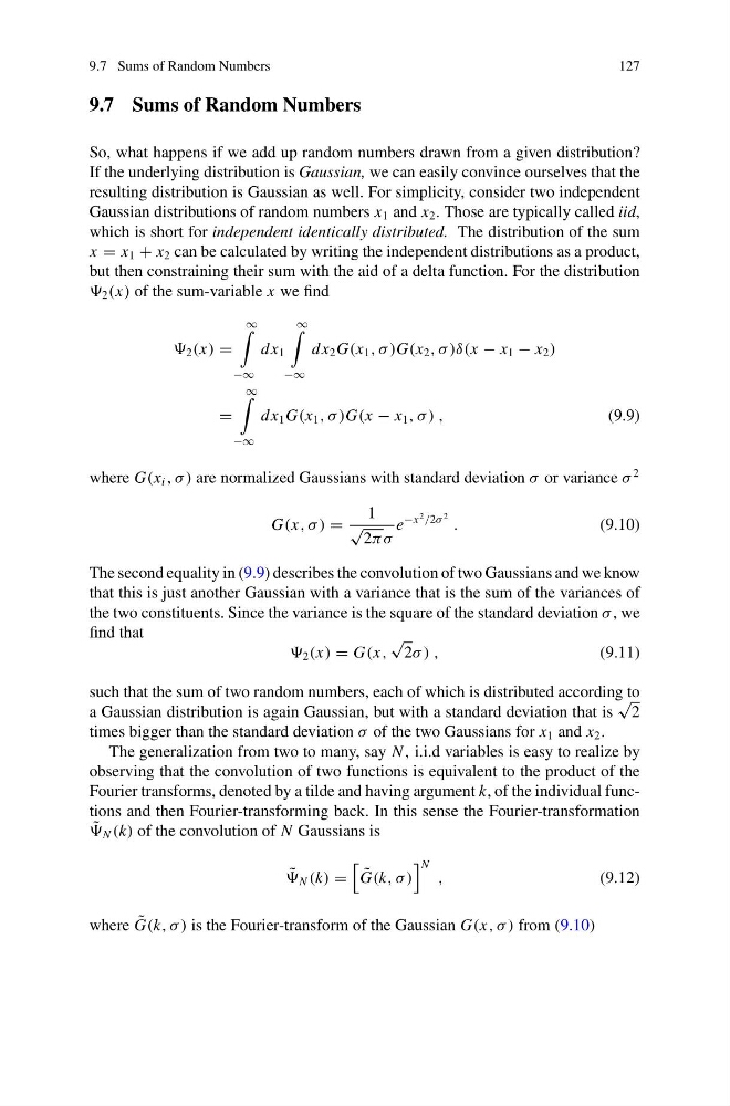
So, what happens if we add up random numbers drawn from a given distribution?
If the underlying distribution is Gaussian, we can easily convince ourselves that the
resulting distribution is Gaussian as well. For simplicity, consider two independent
Gaussian distributions of random numbers x 1 and x 2 . Those are typically called iid,
which is short for independent identically distributed. The distribution of the sum
x = x 1 + x 2 can be calculated by writing the independent distributions as a product,
but then constraining their sum with the aid of a delta function. For the distribution
2 (x) of the sum-variable x we find
2 (x) =
∞
−∞
dx 1
∞
−∞
dx 2 G(x 1 , σ )G(x 2 , σ )δ(x − x 1 − x 2 )
=
∞
−∞
dx 1 G(x 1 , σ )G(x − x 1 , σ ) ,
(9.9)
where G(x i , σ ) are normalized Gaussians with standard deviation σ or variance σ
2
G(x, σ ) =
1
√
2πσ
e
−x
2 /2σ
2 .
(9.10)
The second equality in (9.9) describes the convolution of two Gaussians and we know
that this is just another Gaussian with a variance that is the sum of the variances of
the two constituents. Since the variance is the square of the standard deviation σ , we
find that
2 (x) = G(x,
√
2σ ) ,
(9.11)
such that the sum of two random numbers, each of which is distributed according to
a Gaussian distribution is again Gaussian, but with a standard deviation that is
√
2
times bigger than the standard deviation σ of the two Gaussians for x 1 and x 2 .
The generalization from two to many, say N , i.i.d variables is easy to realize by
observing that the convolution of two functions is equivalent to the product of the
Fourier transforms, denoted by a tilde and having argument k, of the individual functions and then Fourier-transforming back. In this sense the Fourier-transformation
˜
N (k) of the convolution of N Gaussians is
˜
N (k) =
˜
G(k, σ )
N ,
(9.12)
where ˜
G(k, σ ) is the Fourier-transform of the Gaussian G(x, σ ) from (9.10)
127
9.7 Sums of Random Numbers
So, what happens if we add up random numbers drawn from a given distribution?
If the underlying distribution is Gaussian, we can easily convince ourselves that the
resulting distribution is Gaussian as well. For simplicity, consider two independent
Gaussian distributions of random numbers x 1 and x 2 . Those are typically called iid,
which is short for independent identically distributed. The distribution of the sum
x = x 1 + x 2 can be calculated by writing the independent distributions as a product,
but then constraining their sum with the aid of a delta function. For the distribution
2 (x) of the sum-variable x we find
2 (x) =
∞
−∞
dx 1
∞
−∞
dx 2 G(x 1 , σ )G(x 2 , σ )δ(x − x 1 − x 2 )
=
∞
−∞
dx 1 G(x 1 , σ )G(x − x 1 , σ ) ,
(9.9)
where G(x i , σ ) are normalized Gaussians with standard deviation σ or variance σ
2
G(x, σ ) =
1
√
2πσ
e
−x
2 /2σ
2 .
(9.10)
The second equality in (9.9) describes the convolution of two Gaussians and we know
that this is just another Gaussian with a variance that is the sum of the variances of
the two constituents. Since the variance is the square of the standard deviation σ , we
find that
2 (x) = G(x,
√
2σ ) ,
(9.11)
such that the sum of two random numbers, each of which is distributed according to
a Gaussian distribution is again Gaussian, but with a standard deviation that is
√
2
times bigger than the standard deviation σ of the two Gaussians for x 1 and x 2 .
The generalization from two to many, say N , i.i.d variables is easy to realize by
observing that the convolution of two functions is equivalent to the product of the
Fourier transforms, denoted by a tilde and having argument k, of the individual functions and then Fourier-transforming back. In this sense the Fourier-transformation
˜
N (k) of the convolution of N Gaussians is
˜
N (k) =
˜
G(k, σ )
N ,
(9.12)
where ˜
G(k, σ ) is the Fourier-transform of the Gaussian G(x, σ ) from (9.10)