

9.5 Power Laws
121
The moments can then be calculated by standard integrals and are given by
x
m
=
∞
ˆ
x
x
m p(x)dx =
α − 1
α − 1 − m
ˆ
x
m
,
(9.3)
where we expressed the constant C by the one found from normalizing the distribution.
Equation 9.3 already reveals some interesting feature of power laws. In order
to have a first moment—the mean—they are required to have α > 2, otherwise the
right-hand side is negative, despite everything on the left-hand side being positive.
Furthermore, the second moment with m = 2 only exists for α > 3. In the same
spirit, for the mth moment x
m
to exists, we must have α > m + 1. Conversely, a
power law distribution x
−α characterized by exponent α only has moments up to
order α − 1.
As an example, we consider the distribution ψ a (x), known as Lorentz, Cauchy,
or Breit-Wigner distribution in different fields
ψ a (x) =
a
π
1
a 2 + x 2 .
(9.4)
The parameter a is qualitatively related to the width of the distribution. Asymptotically, the distribution behaves as x
−α with α = 2 and is known not to have a second
moment, in correspondence with the general discussion in the previous paragraph.
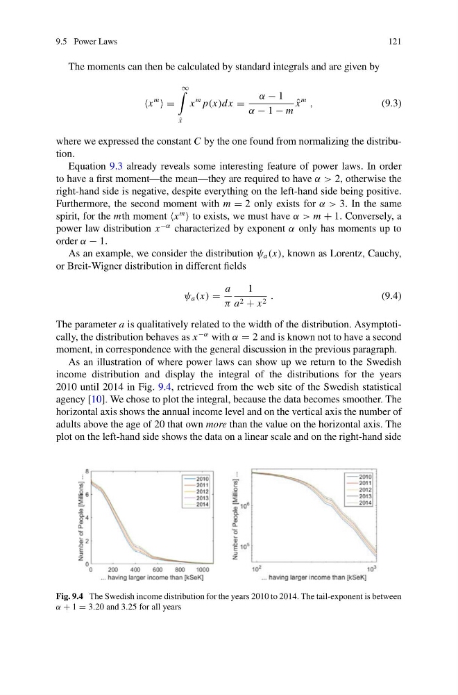
As an illustration of where power laws can show up we return to the Swedish
income distribution and display the integral of the distributions for the years
2010 until 2014 in Fig. 9.4, retrieved from the web site of the Swedish statistical
agency [10]. We chose to plot the integral, because the data becomes smoother. The
horizontal axis shows the annual income level and on the vertical axis the number of
adults above the age of 20 that own more than the value on the horizontal axis. The
plot on the left-hand side shows the data on a linear scale and on the right-hand side
Fig. 9.4 The Swedish income distribution for the years 2010 to 2014. The tail-exponent is between
α + 1 = 3.20 and 3.25 for all years
121
The moments can then be calculated by standard integrals and are given by
x
m
=
∞
ˆ
x
x
m p(x)dx =
α − 1
α − 1 − m
ˆ
x
m
,
(9.3)
where we expressed the constant C by the one found from normalizing the distribution.
Equation 9.3 already reveals some interesting feature of power laws. In order
to have a first moment—the mean—they are required to have α > 2, otherwise the
right-hand side is negative, despite everything on the left-hand side being positive.
Furthermore, the second moment with m = 2 only exists for α > 3. In the same
spirit, for the mth moment x
m
to exists, we must have α > m + 1. Conversely, a
power law distribution x
−α characterized by exponent α only has moments up to
order α − 1.
As an example, we consider the distribution ψ a (x), known as Lorentz, Cauchy,
or Breit-Wigner distribution in different fields
ψ a (x) =
a
π
1
a 2 + x 2 .
(9.4)
The parameter a is qualitatively related to the width of the distribution. Asymptotically, the distribution behaves as x
−α with α = 2 and is known not to have a second
moment, in correspondence with the general discussion in the previous paragraph.
As an illustration of where power laws can show up we return to the Swedish
income distribution and display the integral of the distributions for the years
2010 until 2014 in Fig. 9.4, retrieved from the web site of the Swedish statistical
agency [10]. We chose to plot the integral, because the data becomes smoother. The
horizontal axis shows the annual income level and on the vertical axis the number of
adults above the age of 20 that own more than the value on the horizontal axis. The
plot on the left-hand side shows the data on a linear scale and on the right-hand side
Fig. 9.4 The Swedish income distribution for the years 2010 to 2014. The tail-exponent is between
α + 1 = 3.20 and 3.25 for all years