

108
8 Time Series
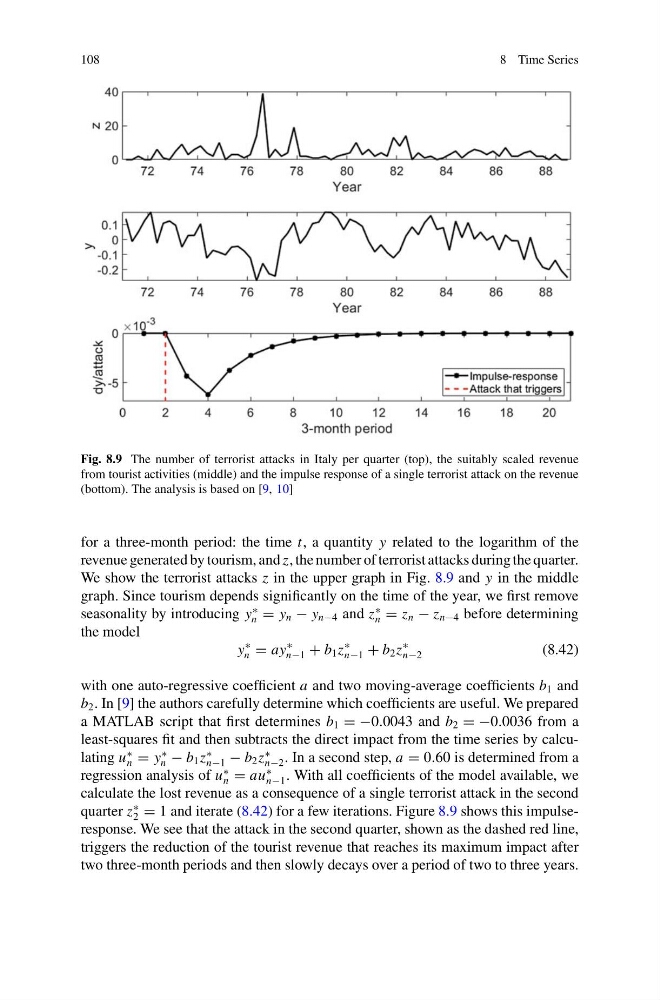
Fig. 8.9 The number of terrorist attacks in Italy per quarter (top), the suitably scaled revenue
from tourist activities (middle) and the impulse response of a single terrorist attack on the revenue
(bottom). The analysis is based on [9, 10]
for a three-month period: the time t, a quantity y related to the logarithm of the
revenue generated by tourism, and z, the number of terrorist attacks during the quarter.
We show the terrorist attacks z in the upper graph in Fig. 8.9 and y in the middle
graph. Since tourism depends significantly on the time of the year, we first remove
seasonality by introducing y
∗
n = y n − y n−4 and z
∗
n = z n − z n−4 before determining
the model
y
∗
n = ay
∗
n−1 + b 1 z
∗
n−1 + b 2 z
∗
n−2
(8.42)
with one auto-regressive coefficient a and two moving-average coefficients b 1 and
b 2 . In [9] the authors carefully determine which coefficients are useful. We prepared
a MATLAB script that first determines b 1 = −0.0043 and b 2 = −0.0036 from a
least-squares fit and then subtracts the direct impact from the time series by calculating u
∗
n = y
∗
n − b 1 z
∗
n−1 − b 2 z
∗
n−2 . In a second step, a = 0.60 is determined from a
regression analysis of u
∗
n = au
∗
n−1 . With all coefficients of the model available, we
calculate the lost revenue as a consequence of a single terrorist attack in the second
quarter z
∗
2 = 1 and iterate (8.42) for a few iterations. Figure 8.9 shows this impulseresponse. We see that the attack in the second quarter, shown as the dashed red line,
triggers the reduction of the tourist revenue that reaches its maximum impact after
two three-month periods and then slowly decays over a period of two to three years.
8 Time Series
Fig. 8.9 The number of terrorist attacks in Italy per quarter (top), the suitably scaled revenue
from tourist activities (middle) and the impulse response of a single terrorist attack on the revenue
(bottom). The analysis is based on [9, 10]
for a three-month period: the time t, a quantity y related to the logarithm of the
revenue generated by tourism, and z, the number of terrorist attacks during the quarter.
We show the terrorist attacks z in the upper graph in Fig. 8.9 and y in the middle
graph. Since tourism depends significantly on the time of the year, we first remove
seasonality by introducing y
∗
n = y n − y n−4 and z
∗
n = z n − z n−4 before determining
the model
y
∗
n = ay
∗
n−1 + b 1 z
∗
n−1 + b 2 z
∗
n−2
(8.42)
with one auto-regressive coefficient a and two moving-average coefficients b 1 and
b 2 . In [9] the authors carefully determine which coefficients are useful. We prepared
a MATLAB script that first determines b 1 = −0.0043 and b 2 = −0.0036 from a
least-squares fit and then subtracts the direct impact from the time series by calculating u
∗
n = y
∗
n − b 1 z
∗
n−1 − b 2 z
∗
n−2 . In a second step, a = 0.60 is determined from a
regression analysis of u
∗
n = au
∗
n−1 . With all coefficients of the model available, we
calculate the lost revenue as a consequence of a single terrorist attack in the second
quarter z
∗
2 = 1 and iterate (8.42) for a few iterations. Figure 8.9 shows this impulseresponse. We see that the attack in the second quarter, shown as the dashed red line,
triggers the reduction of the tourist revenue that reaches its maximum impact after
two three-month periods and then slowly decays over a period of two to three years.