

11.7 Examples Concerning Class LME
425
˙
q L (t; t 0 ) = f L
f MC (σ MC (t; t 0 ) + σ MC 0 )
−f MC (σ MC 0 ) − ϕ e (t; t 0 ) + ϕ L 0
˙
σ MC (t; t 0 ) = −q L (t; t 0 ) + q a (t; t 0 ) + q MC 0
in the state variables q L (t; t 0 ) and σ MC (t; t 0 ).
Using KϕL with the CR of the memcapacitor it can be checked that
d
dt
[ϕ L (t) − f MC (σ MC (t))] = e(t)
(11.38)
for any t ≥ t 0 .
Hence, the three-dimensional state space (ϕ L , σ MC , q MC ) ∈ R 3 can be decomposed in ∞ 1 1D manifolds, which are (positively) invariant for the dynamics in the
(v, i)-domain, given by
M(Φ 0 ) = {(σ MC (t), q MC (t), ϕ L (t))
T
∈ R
3
:
ϕ L (t) − f MC (σ MC (t)) = Φ 0 }
where Φ 0 ∈ R. On each manifold the dynamics is second order and can be described
by the corresponding SE in the (ϕ, q)-domain. This also implies that there coexist
∞ 1 different second-order dynamics, one for each manifold, in the (v, i)-domain.
Due to (11.38), it is seen that manifolds can be programmed via the voltage
source e(t), while the current source a(t) has no effect on manifold programming.
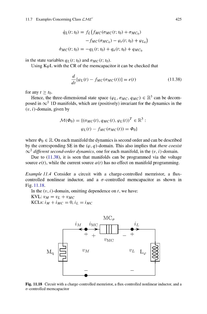
Example 11.4 Consider a circuit with a charge-controlled memristor, a fluxcontrolled nonlinear inductor, and a σ -controlled memcapacitor as shown in
Fig. 11.18.
In the (v, i)-domain, omitting dependence on t, we have:
KVL: v M = v L + v MC
KCLs: i M + i MC = 0, i L = i MC
Fig. 11.18 Circuit with a charge-controlled memristor, a flux-controlled nonlinear inductor, and a
σ -controlled memcapacitor
425
˙
q L (t; t 0 ) = f L
f MC (σ MC (t; t 0 ) + σ MC 0 )
−f MC (σ MC 0 ) − ϕ e (t; t 0 ) + ϕ L 0
˙
σ MC (t; t 0 ) = −q L (t; t 0 ) + q a (t; t 0 ) + q MC 0
in the state variables q L (t; t 0 ) and σ MC (t; t 0 ).
Using KϕL with the CR of the memcapacitor it can be checked that
d
dt
[ϕ L (t) − f MC (σ MC (t))] = e(t)
(11.38)
for any t ≥ t 0 .
Hence, the three-dimensional state space (ϕ L , σ MC , q MC ) ∈ R 3 can be decomposed in ∞ 1 1D manifolds, which are (positively) invariant for the dynamics in the
(v, i)-domain, given by
M(Φ 0 ) = {(σ MC (t), q MC (t), ϕ L (t))
T
∈ R
3
:
ϕ L (t) − f MC (σ MC (t)) = Φ 0 }
where Φ 0 ∈ R. On each manifold the dynamics is second order and can be described
by the corresponding SE in the (ϕ, q)-domain. This also implies that there coexist
∞ 1 different second-order dynamics, one for each manifold, in the (v, i)-domain.
Due to (11.38), it is seen that manifolds can be programmed via the voltage
source e(t), while the current source a(t) has no effect on manifold programming.
Example 11.4 Consider a circuit with a charge-controlled memristor, a fluxcontrolled nonlinear inductor, and a σ -controlled memcapacitor as shown in
Fig. 11.18.
In the (v, i)-domain, omitting dependence on t, we have:
KVL: v M = v L + v MC
KCLs: i M + i MC = 0, i L = i MC
Fig. 11.18 Circuit with a charge-controlled memristor, a flux-controlled nonlinear inductor, and a
σ -controlled memcapacitor