

9.2 Memristor Neural Network Model
353
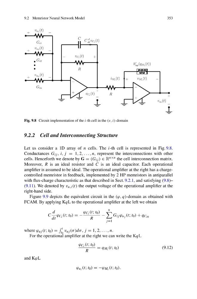
Fig. 9.8 Circuit implementation of the i-th cell in the (v, i)-domain
9.2.2 Cell and Interconnecting Structure
Let us consider a 1D array of n cells. The i-th cell is represented in Fig. 9.8.
Conductances G ij , i, j = 1, 2, . . . , n, represent the interconnections with other
cells. Henceforth we denote by G = (G ij ) ∈ R n×n the cell interconnection matrix.
Moreover, R is an ideal resistor and C is an ideal capacitor. Each operational
amplifier is assumed to be ideal. The operational amplifier at the right has a chargecontrolled memristor in feedback, implemented by 2 HP memristors in antiparallel
with flux-charge characteristic as that described in Sect. 9.2.1, and satisfying (9.8)–
(9.11). We denoted by v u,i (t) the output voltage of the operational amplifier at the
right-hand side.
Figure 9.9 depicts the equivalent circuit in the (ϕ, q)-domain as obtained with
FCAM. By applying KqL to the operational amplifier at the left we obtain
C
d
dt
ϕ C i (t; t 0 ) = −
ϕ C i (t; t 0 )
R
−
n
j =1
G ij ϕ u j (t; t 0 ) + q C i0
where ϕ uj (t; t 0 ) =
t
t 0
v uj (σ )dσ , j = 1, 2, . . . , n.
For the operational amplifier at the right we can write the KqL
ϕ C i (t; t 0 )
R
= q M i (t; t 0 )
(9.12)
and KϕL
ϕ u i (t; t 0 ) = −ϕ M i (t; t 0 ).
353
Fig. 9.8 Circuit implementation of the i-th cell in the (v, i)-domain
9.2.2 Cell and Interconnecting Structure
Let us consider a 1D array of n cells. The i-th cell is represented in Fig. 9.8.
Conductances G ij , i, j = 1, 2, . . . , n, represent the interconnections with other
cells. Henceforth we denote by G = (G ij ) ∈ R n×n the cell interconnection matrix.
Moreover, R is an ideal resistor and C is an ideal capacitor. Each operational
amplifier is assumed to be ideal. The operational amplifier at the right has a chargecontrolled memristor in feedback, implemented by 2 HP memristors in antiparallel
with flux-charge characteristic as that described in Sect. 9.2.1, and satisfying (9.8)–
(9.11). We denoted by v u,i (t) the output voltage of the operational amplifier at the
right-hand side.
Figure 9.9 depicts the equivalent circuit in the (ϕ, q)-domain as obtained with
FCAM. By applying KqL to the operational amplifier at the left we obtain
C
d
dt
ϕ C i (t; t 0 ) = −
ϕ C i (t; t 0 )
R
−
n
j =1
G ij ϕ u j (t; t 0 ) + q C i0
where ϕ uj (t; t 0 ) =
t
t 0
v uj (σ )dσ , j = 1, 2, . . . , n.
For the operational amplifier at the right we can write the KqL
ϕ C i (t; t 0 )
R
= q M i (t; t 0 )
(9.12)
and KϕL
ϕ u i (t; t 0 ) = −ϕ M i (t; t 0 ).